The
Bias-Variance trade-off is a basic yet important concept in the field of
data science and machine learning. Often, we encounter statements like
“simpler models have high bias and low variance whereas more complex or
sophisticated models have low bias and high variance” or “high bias
leads to under-fitting and high variance leads to over-fitting”. But
what do bias and variance actually mean and how are they related to the
accuracy and performance of a model?
In
this article, I will explain the intuitive and mathematical meaning of
bias and variance, show the mathematical relation between bias, variance
and performance of a model and finally demo the effects of varying the
model complexity on bias and variance through a small example.
Assumptions to start with
Bias
and variance are statistical terms and can be used in varied contexts.
However, in this article, they will be discussed in terms of an
estimator which is trying to fit/explain/estimate some unknown data
distribution.
Before we delve into the bias and variance of an estimator, let us assume the following :-
- There is a data generator, Y = f(X) + ϵ, which is generating Data(X,Y), where ϵ is the added random gaussian noise, centered at origin with some standard deviation σ i.e. E[ϵ] = 0 and Var(ϵ) = σ² . Note that data can be sampled repetitively from the generator yielding different sample sets say Xᵢ , Yᵢ on iᵗʰ iteration.
- We are trying to estimate(fit a curve) to the sample set we have available from the generator, using an estimator. An estimator usually is a class of models like Ridge regressor, Decision Tree or Support Vector Regressor etc. A class of models can be represented as g(X/θ) where θ are the parameters. For different values of θ, we get different models within that particular class of models and we try vary θ to find the best fitting model for our sample set.
Meaning of Bias and Variance
Bias
of an estimator is the the “expected” difference between its estimates
and the true values in the data. Intuitively, it is a measure of how
“close”(or far) is the estimator to the actual data points which the
estimator is trying to estimate. Notice that I have used the word
“expected” which implies that the difference is being thought over
keeping in mind that we will be doing this model training experiment
(ideally)infinite number of times. Each of those models will be trained
on different sample sets Xᵢ , Yᵢ of the true data resulting in their
parameters taking different values of θ in a bid to explain/fit/estimate
that particular sample best.
Eventually for some test point xₒ , the bias of this estimator g(X) can be mathematically written as :-
Bias[g(xₒ)] = E[g(xₒ)] − f(xₒ)
which is literally the difference between the expected value of an estimator at that point and the true value at that same point.
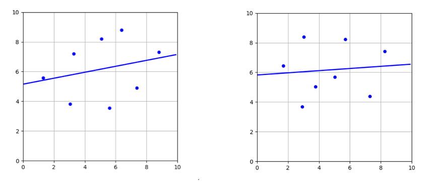
Naturally, an estimator will have high bias
at a test point(and hence overall too, in the limit) if it does NOT
wiggle or change too much when a different sample set of the data is
thrown at it. This will usually be the case when an estimator does not
have enough “capacity” to adequately fit the inherent data generating
function. Therefore, simpler models have a higher bias compared to more
sophisticated models.
Hold these thoughts and we will come back to them again later in the article. For now, here is a figure to help solidify them a bit more.

Variance of
an estimator is the “expected” value of the squared difference between
the estimate of a model and the “expected” value of the estimate(over
all the models in the estimator). Too convoluted to understand in a go? Lets break that sentence down..
Suppose
we are training ∞ models using different sample sets of the data. Then
at a test point xₒ, the expected value of the estimate over all those
models is the E[g(xₒ)]. Also, for any individual model out of all the
models, the estimate of that model at that point is g(xₒ). The
difference between these two can be written as g(xₒ) − E[g(xₒ)].
Variance is the expected value of the square of this distance over all
the models. Hence, variance of the estimator at at test point xₒ can be
mathematically written as :-
Var[g(xₒ)] = E[(g(xₒ) − E[g(xₒ)])²]
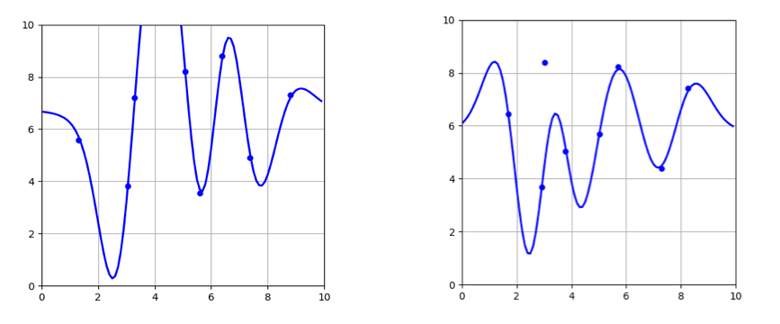
Going by this equation, we can say that an estimator has high variance
when the estimator “varies” or changes its estimate a lot at any data
point, when it is trained over different sample sets of the data.
Another way to put this is that the estimator is flexible/sophisticated
enough, or has a high “capacity” to perfectly fit/explain/estimate the
training sample set given to it due to which its value at other points
fluctuates immensely.

Notice
that this interpretation of the meaning of high variance is exactly
opposite to that of an estimator having high bias. This implies that bias
and variance of an estimator are complementary to each other i.e. an
estimator with high bias will vary less(have low variance) and an
estimator with high variance will have less bias(as it can vary more to
fit/explain/estimate the data points).
The Bias-Variance Decomposition
In
this section, we see how the bias and variance of an estimator are
mathematically related to each other and also to the performance of the
estimator. We will start with defining estimator’s error at a test point
as the “expected” squared difference between the true value and
estimator’s estimate.
By
now, it should be fairly clear that whenever we are talking about an
expected value, we are referring to the expectation over all the
possible models, trained individually over all the possible data samples
from the data generator. For any unseen test point xₒ, we have :-
Err(xₒ) = E[(Y − g(xₒ))² | X = xₒ]
For notational simplicity, I am referring to f(xₒ) and g(xₒ) as f and g respectively and skipping the conditional on X :-
Err(xₒ) = E[(Y − g(xₒ))²]
= E[(f + ϵ − g)²]
= E[ϵ²] + E[(f − g)²] + 2.E[(f − g)ϵ]
= E[(ϵ − 0)²] + E[(f − E[g] + E[g] − g)²] + 2.E[fϵ] − 2.E[gϵ]
= E[(ϵ − E[ϵ])²] + E[(f − E[g] + E[g] − g)²] + 0 − 0
= Var(ϵ) + E[(g − E[g])²] + E[(E[g] − f)²] + 2.E[(g − E[g])(E[g] − f)]
= Var(ϵ) + Var(g) + Bias(g)² + 2.{E[g]² − E[gf] − E[g]² + E[gf]}
= σ² + Var(g) + Bias(g)²
- So, the error(and hence the accuracy) of the estimator at an unseen data sample xₒ can be decomposed into variance of the noise in the data, bias and the variance of the estimator. This implies that both bias and variance are the sources of error of an estimator.
- Also, in the previous section we have seen that bias and variance of an estimator are complementary to each other i.e. the increasing one of them would mean a decrease in the other and vice versa.
Now pause for a bit and try thinking a bit about what these two facts coupled together could mean for an estimator….
The Bias-Variance Trade-off
From
the complementary nature of bias and variance and estimator’s error
decomposing into bias and variance, it is clear that there is a
trade-off between bias and variance when it comes to the performance of
the estimator.
An
estimator will have a high error if it has very high bias and low
variance i.e. when it is not able to adapt at all to the data points in a
sample set. On the other extreme, an estimator will also have a high
error if it has very high variance and low bias i.e. when it adapts too
well to all the data points in a sample set(a sample set is an
incomplete representation of true data) and hence fails to generalize
other unseen samples and eventually fails to generalize the true
dataset.
An
estimator that strikes a balance between the bias and variance is able
to minimize the error better than those that live on extreme ends.
Although it is beyond the scope of this article, this can be proved
using basic differential calculus.

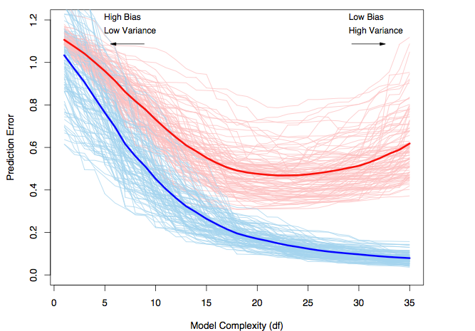
This figure has been taken from ESLR
and it explains the trade-off very well. In this example, 100 sample
sets of size 50 have been used to train 100 models of the same class,
each of whose complexity/capacity is being increased from left to right.
Each individual light blue curve belongs to a model and demonstrates
how the model’s training set error changes as the complexity of the
model is increased. Every point on the light red curve in turn is the
model’s error on a common test set, tracing the curve as the complexity
of the model is varied. Finally, the darker curves are the respective
average(tending to expected value in the limit) training and test set
errors. We can see that the models that strike a balance between bias
and variance are able to generalize the best and perform substantially
better than those with high bias or high variance.
Demo
I
have put up a small demo showing everything I have talked about in this
article. If all of this makes sense and you would like to try it out on
your own, do check it out below! I have compared the bias-variance
tradeoff between Ridge regressor and K-Nearest Neighbor Regressor with K
= 1.
Keep
in mind that KNN Regressor, K = 1 fits the training set perfectly so it
“varies” a lot when the training set is changed while Ridge regressor
does not.
I
hope this article explained the concept well and was fun to read! If
you have any follow up questions, please post a comment and I will try
to answer them.
No comments:
Post a Comment