These days I come across many people who want to get into machine
learning/AI, particularly deep learning. Some are asking me what the
best way is to get started and learn. Clearly, at the speed things are
evolving, there seems to be no time for a PhD. Universities are
sometimes a bit behind the curve on applications, technology and
infrastructure, so is a masters worth doing? A couple companies now
offer residency programmes, extended internships, which supposedly allow
you to kickstart a successful career in machine learning without a PhD.
What your best option is depends largely on your circumstances, but
also on what you want to achieve.
Just too easy
The general advice I increasingly find myself giving is this: deep
learning is too easy. Pick something harder to learn, learning deep
learning should not be the goal but a side effect.
Deep learning is powerful exactly because it makes hard things easy.
The reason deep learning made such a splash is the very fact that it
allows us to phrase several previously impossible learning problems as
empirical loss minimisation via gradient descent, a conceptually super
simple thing. Deep networks deal with natural signals we previously had
no easy ways of dealing with: images, video, human language, speech,
sound. But almost whatever you do in deep learning, at the end of the
day it becomes super simple: you combine a couple basic building blocks
and ideas (convolution, pooling, recurrence), you can do it without
overthinking it, if you have enough data the network will figure it out.
Increasingly high-level, declarative frameworks like TensorFlow,
Theano, Lasagne, Blocks, Keras, etc simplify this to the level of
building Lego towers.
Pick something harder
This is not to say there are no genuinely novel ideas coming out of
deep learning, or using deep learning in more innovative ways, far from
it. Generative Adversarial Networks and Variational Autoencoders are
brilliant examples that sparked new interest in probabilistic/generative
modelling. Understanding why/how those work, and how to
generalise/build on them is real hard - the deep learning bit is easy.
There is not much low-hanging fruit left for deep learning.
Supervised learning - while still being improved - is now considered
largely solved and boring. Unsupervised learning will certainly benefit
from the deep learning toolkit, but it also requires a very different
kind of thinking, familiarity with information
theory/probabilities/geometry. Insight into how to make these methods
actually work are unlikely to come in the form of improvements to neural
network architectures.
What I'm saying is that by learning deep learning, most
people mean learning to use a relatively simple toolbox. But in six
months time, many, many more people will have those skills. Don't spend
time working on/learning about stuff that retrospectively turns out to
be too easy. You might miss your chance to make a real impact with your
work and differentiate your career in the long term. Think about what
you really want to be able to learn, pick something harder, and then go
work with people who can help you with that.
Back to basics
What are examples of harder things to learn? Consider what knowledge
authors like Ian Goodfellow, Durk Kingma, etc have used when they came
up with the algorithms mentioned before. Much of the relevant stuff that
is now being rediscovered was actively researched in the early 2000's.
Learn classic things like the EM algorithm, variational inference, unsupervised learning with linear Gaussian systems:
PCA, factor analysis, Kalman filtering, slow feature analysis. I can
also recommend Aapo Hyvarinen's work on ICA, pseudolikelihood. You
should try to read (and understand) the original deep belief network
paper.
Shortcut to the next frontiers
While deep learning is where most interesting breakthroughs happened
recently, it's worth trying to bet on areas that might gain relevance
going forward:
probabilistic programming and black-box probabilistic inference (with- or without deep neural networks). Take a look at Picture for example, or Josh Tenenbaum's work on inverse graphics networks. Or stuff at this NIPS workshop on black-box inference. To quote my colleague Lucas Theis:
probabilistic programming could do for Bayesian ML what Theano has done for neural networks
better/scaleable MCMC and variational inference methods, again,
with or without the use of deep neural networks. There is a lot of
recent work on things like this. Again, if we made MCMC as reliable as
stochastic gradient descent now is for deep networks, that could mean a
resurgence of more explicit Bayesian/probabilistic models and
hierarchical graphical models, of which RBMs are just one example.
Have I seen this before?
Roughly the same thing happened around the data scientist
buzzword some years ago. Initially, using Hadoop, Hive, etc were a big
deal, and several early adopters made a very successful career out of -
well - being early adopters. Early on, all you really needed to do was
counting stuff on smallish distributed clusters, and you quickly
accumulated tens of thousands of followers who worshipped you for being a
big data pioneer.
What people did back then seemed magic at the time, but looking back
from just a couple years it's trivial: lots of people use Hadoop and
spark now, and tools like Amazon's Redshift made stuff even simpler.
Back in the days, your startup could get funded on the premise that your
team could use Hive, but unless you used it in some interesting way,
that technological advantage evaporated very quickly. At the top of the
hype cycle, there were data science internships, residential
training programs, bootcamps, etc. By the time people graduated from
these programs, these skills were rendered somewhat irrelevant and
trivial. What is happening now with deep learning looks very similar.
In summary, if you are about to get into deep learning, just
think about what that means, and try to be more specific. Think about
how many other people are in your position right now, and how are you
going to make sure the things you learn aren't the ones that will appear
super-boring in a year's time.
Microsoft is making the tools that its own researchers use to speed
up advances in artificial intelligence available to a broader group of
developers by releasing its Computational Network Toolkit on GitHub.
The researchers developed the open-source toolkit, dubbed CNTK, out of necessity. Xuedong Huang, Microsoft’s chief speech scientist, said he and his team were anxious to make faster improvements to how well computers can understand speech, and the tools they had to work with were slowing them down.
So, a group of volunteers set out to solve this problem on their own,
using a homegrown solution that stressed performance over all else.
The effort paid off.
In internal tests, Huang said CNTK has proved more efficient
than four other popular computational toolkits that developers use to
create deep learning models for things like speech and image
recognition, because it has better communication capabilities
“The CNTK toolkit is just insanely more efficient than anything we have ever seen,” Huang said.
Those types of performance gains are incredibly important in the
fast-moving field of deep learning, because some of the biggest deep
learning tasks can take weeks to finish. Over
the past few years, the field of deep learning has exploded as more
researchers have started running machine learning algorithms using deep
neural networks, which are systems that are inspired by the biological
processes of the human brain. Many researchers see deep learning as a
very promising approach for making artificial intelligence better.
Those gains have allowed researchers to create systems that can accurately recognize and even translate conversations, as well as ones that can recognize images and even answer questions about them.
Internally, Microsoft is using CNTK on a set of powerful computers that use graphics processing units, or GPUs.
Although GPUs were designed for computer graphics, researchers have
found that they also are ideal for processing the kind of algorithms
that are leading to these major advances in technology that can speak,
hear and understand speech, and recognize images and movements.
Chris Basoglu, a principal development manager at Microsoft who also
worked on the toolkit, said one of the advantages of CNTK is that it can
be used by anyone from a researcher on a limited budget, with a single
computer, to someone who has the ability to create their own large
cluster of GPU-based computers. The researchers say it can scale across
more GPU-based machines than other publicly available toolkits,
providing a key advantage for users who want to do large-scale
experiments or calculations.
Xuedong Huang (Photography by Scott Eklund/Red Box Pictures)
Huang said it was important for his team to be able to address
Microsoft’s internal needs with a tool like CNTK, but they also want to
provide the same resources to other researchers who are making similar
advances in deep learning.
That’s why they decided to make the tools available via open source licenses to other researchers and developers.
Last April, the researchers made the toolkit available to academic researchers, via Codeplex and under a more restricted open-source license.
But starting Monday it also will be available, via an open-source
license, to anyone else who wants to use it. The researchers say it
could be useful to anyone from deep learning startups to more
established companies that are processing a lot of data in real time.
“With CNTK, they can actually join us to drive artificial intelligence breakthroughs,” Huang said.
Neural networks have seen spectacular progress during the last
few years and they are now the state of the art in image recognition and
automated translation. TensorFlow
is a new framework released by Google for numerical computations and
neural networks. In this blog post, we are going to demonstrate how to
use TensorFlow and Spark together to train and apply deep learning
models.
You might be wondering: what’s Spark’s use here when most
high-performance deep learning implementations are single-node only? To
answer this question, we walk through two use cases and explain how you
can use Spark and a cluster of machines to improve deep learning
pipelines with TensorFlow:
Hyperparameter Tuning: use Spark to find the best set of
hyperparameters for neural network training, leading to 10X reduction in
training time and 34% lower error rate.
Deploying models at scale: use Spark to apply a trained neural network model on a large amount of data.
Hyperparameter Tuning
An example of a deep learning machine learning (ML) technique is
artificial neural networks. They take a complex input, such as an image
or an audio recording, and then apply complex mathematical transforms on
these signals. The output of this transform is a vector of numbers that
is easier to manipulate by other ML algorithms. Artificial neural
networks perform this transformation by mimicking the neurons in the
visual cortex of the human brain (in a much-simplified form).
Just as humans learn to interpret what they see, artificial neural
networks need to be trained to recognize specific patterns that are
‘interesting’. For example, these can be simple patterns such as edges,
circles, but they can be much more complicated. Here, we are going to use a classical dataset put together by NIST and train a neural network to recognize these digits:
The TensorFlow library automates the creation of training algorithms
for neural networks of various shapes and sizes. The actual process of
building a neural network, however, is more complicated than just
running some function on a dataset. There are typically a number of very
important hyperparameters (configuration parameters in layman’s terms)
to set, which affects how the model is trained. Picking the right
parameters leads to high performance, while bad parameters can lead to
prolonged training and bad performance. In practice, machine learning
practitioners rerun the same model multiple times with different
hyperparameters in order to find the best set. This is a classical
technique called hyperparameter tuning.
When building a neural network, there are many important hyperparameters to choose carefully. For example:
Number of neurons in each layer: Too few neurons will reduce the
expression power of the network, but too many will substantially
increase the running time and return noisy estimates.
Learning rate: If it is too high, the neural network will only focus
on the last few samples seen and disregard all the experience
accumulated before. If it is too low, it will take too long to reach a
good state.
The interesting thing here is that even though TensorFlow itself is
not distributed, the hyperparameter tuning process is “embarrassingly
parallel” and can be distributed using Spark. In this case, we can use
Spark to broadcast the common elements such as data and model
description, and then schedule the individual repetitive computations
across a cluster of machines in a fault-tolerant manner.
How does using Spark improve the accuracy? The accuracy with the default set of hyperparameters is 99.2%. Our best result with hyperparameter tuning has a 99.47% accuracy on the test set, which is a 34% reduction of the test error.
Distributing the computations scaled linearly with the number of nodes
added to the cluster: using a 13-node cluster, we were able to train 13
models in parallel, which translates into a 7x speedup compared
to training the models one at a time on one machine. Here is a graph of
the computation times (in seconds) with respect to the number of
machines on the cluster:
More important though, we get insights into the sensibility of the
training procedure to various hyperparameters of training. For example,
we plot the final test performance with respect to the learning rate,
for different numbers of neurons:
This shows a typical tradeoff curve for neural networks:
The learning rate is critical: if it is too low, the neural network
does not learn anything (high test error). If it is too high, the
training process may oscillate randomly and even diverge in some
configurations.
The number of neurons is not as important for getting a good
performance, and networks with many neurons are much more sensitive to
the learning rate. This is Occam’s Razor principle: simpler model tend
to be “good enough” for most purposes. If you have the time and resource
to go after the missing 1% test error, you must be willing to invest a
lot of resources in training, and to find the proper hyperparameters
that will make the difference.
By using a sparse sample of parameters, we can zero in on the most promising sets of parameters.
How do I use it?
Since TensorFlow can use all the cores on each worker, we only run
one task at one time on each worker and we batch them together to limit
contention. The TensorFlow library can be installed on Spark clusters as
a regular Python library, following the instructions on the TensorFlow website. The following notebooks below show how to install TensorFlow and let users rerun the experiments of this blog post:
TensorFlow models can directly be embedded within pipelines to
perform complex recognition tasks on datasets. As an example, we show
how we can label a set of images from a stock neural network model that was already trained.
The model is first distributed to the workers of the clusters, using Spark’s built-in broadcasting mechanism:
1
2
3
withgfile.FastGFile( 'classify_image_graph_def.pb', 'rb') as f:
model_data =f.read()
model_data_bc =sc.broadcast(model_data)
Then this model is loaded on each node and applied to images. This is a sketch of the code being run on each node:
1
2
3
4
5
6
7
8
9
10
11
12
13
14
15
defapply_batch(image_url):
#Creates a newTensorFlow graph of computation and imports the model
This code can be made more efficient by batching the images together.
Here is an example of image:
And here is the interpretation of this image according to the neural network, which is pretty accurate:
We have shown how to combine Spark and TensorFlow to train and deploy
neural networks on handwritten digit recognition and image labeling.
Even though the neural network framework we used itself only works in a
single-node, we can use Spark to distribute the hyperparameter tuning
process and model deployment. This not only cuts down the training
time but also improves accuracy and gives us a better understanding of
various hyperparameters’ sensibility.
While this support is only available on Python, we look forward to
providing deeper integration between TensorFlow and the rest of the
Spark framework.
It
is hard not to be enamoured by deep learning nowadays, watching neural
networks show off their endless accumulation of new tricks. There are,
as I see it, at least two good reasons to be impressed: (1) Neural networks can learn to model many natural functions well, from weak priors. The
idea of marrying hierarchical, distributed representations with fast,
GPU-optimised gradient calculations has turned out to be very powerful
indeed. The early days of neural networks saw problems with local
optima, but the ability to train deeper networks has solved this
and allowed backpropagation to shine through. After baking in a small
amount of domain knowledge through simple architectural decisions, deep
learning practitioners now find themselves with a powerful class of
parameterised functions and a practical way to optimise them.
The first such architectural decisions were the use of either
convolutions or recurrent structure, to imbue models with spatial and
temporal invariances. From this alone, neural networks excelled in image
classification, speech recognition, machine translation, atari games,
and many more domains. More recently, mechanisms for top-down attention
over inputs have shown their worth in image and natural language tasks, while differentiable memory modules such as tapes and stacks have even enabled networks to learn the rules of simple algorithms from only input-output pairs. (2) Neural networks can learn surprisingly useful representations While
the community still waits eagerly for unsupervised learning to bear
fruit, deep supervised learning has shown an impressive aptitude for
building generalisable and interpretable features. That is to say, the
features learned when a neural network is trained to predict P(y|x)
often turn out to be both semantically interpretable and useful for
modelling some other related function P(z|x).
As just a few examples of this:
Units of a convolutional network trained to classify scenes
often learn to detect specific objects in those scenes (such as a
lighthouse), even though they were not explicitly trained to do so (Bolei et al., 2015)
Correlations in the bottom layers of an image classification network
provide a surprisingly good signature for the artistic style of an
image, allowing new images to be synthesised using the content of one
and the style of another (Gatys et al., 2015)
A recurrent network[correction below] taught
to predict missing words from sentences learns meaningful word
embeddings, where simple vector arithmetic can be used to find semantic
analogies. For example:
vking - vman + vwoman ≈ vqueen
vParis - vFrance + vItaly ≈ vRome
vWindows - vMicrosoft + vGoogle ≈ vAndroid
I have no doubt that the next few years will see neural networks
turn their attention to yet more tasks, integrate themselves more
deeply into industry, and continue to impress researchers with new
superpowers. This is all well justified, and I have no intention to
belittle the current and future impact of deep learning; however, the
optimism about the just what these models can achieve in terms of intelligence has been worryingly reminiscent of the 1960s.
Extrapolating from the last few years’ progress, it is enticing to believe that Deep Artificial General Intelligence
is just around the corner and just a few more architectural tricks,
bigger data sets and faster computing power are required to take us
there. I feel that there are a couple of solid reasons to be much more
skeptical.
To begin with, it is a bad idea to intuit how broadly intelligent a
machine must be, or have the capacity to be, based solely on a single
task. The checkers-playing machines of the 1950s amazed researchers and
many considered these a huge leap towards human-level reasoning, yet we
now appreciate that achieving human or superhuman performance in this
game is far easier than achieving human-level general intelligence. In
fact, even the best humans can easily be defeated by a search algorithm
with simple heuristics. The development of such an algorithm probably
does not advance the long term goals of machine intelligence, despite
the exciting intelligent-seeming behaviour it gives rise to,
and the same could be said of much other work in artificial intelligence
such as the expert systems of the 1980s. Human or superhuman
performance in one task is not necessarily a stepping-stone towards
near-human performance across most tasks.
By the same token, the ability of neural networks to learn
interpretable word embeddings, say, does not remotely suggest that they
are the right kind of tool for a human-level understanding of the world.
It is impressive and surprising that these general-purpose, statistical
models can learn meaningful relations from text alone, without any
richer perception of the world, but this may speak much more about the
unexpected ease of the task itself than it does about the capacity of
the models. Just as checkers can be won through tree-search, so too can
many semantic relations be learned from text statistics. Both produce
impressive intelligent-seeming behaviour, but neither necessarily pave the way towards true machine intelligence.
I’d like to reflect on specifically what neural networks are good at,
and how this relates to human intelligence. Deep learning has produced
amazing discriminative models, generative models and feature extractors,
but common to all of these is the use of a very large training dataset.
Its place in the world is as a powerful tool for general-purpose
pattern recognition, in situations where n and d are high. Very possibly it is the best tool for working in this paradigm.
This is a very good fit for one particular class of problems that the
brain solves: finding good representations to describe the constant and
enormous flood of sensory data it receives. Before any sense can be
made of the environment, the visual and auditory systems need to fold,
stretch and twist this data from raw pixels and waves into a form that
better captures the complex statistical regularities in the signal*.
Whether this is learned from scratch or handed down as a gift from
evolution, the brain solves this problem adeptly - and there is even recent evidence that
the representations it finds are not too dissimilar from those
discovered by a neural network. I contend, deep learning may well
provide a fantastic starting point for many problems in perception.
That said, this high n, high d paradigm is a very
particular one, and is not the right environment to describe a great
deal of intelligent behaviour. The many facets of human thought include
planning towards novel goals, inferring others' goals from their
actions, learning structured theories to describe the rules of the
world, inventing experiments to test those theories, and learning to
recognise new object kinds from just one example. Very often they
involve principled inference under uncertainty from few observations.
For all the accomplishments of neural networks, it must be said that
they have only ever proven their worth at tasks fundamentally different
from those above. If they have succeeded in anything superficially
similar, it has been because they saw many hundreds of times more
examples than any human ever needed to.
Deep learning has brought us one branch higher up the tree towards
machine intelligence and a wealth of different fruit is now hanging
within our grasp. While the ability to learn good features in high
dimensional spaces from weak priors with lots of data is both new and
exciting, we should not fall into the trap of thinking that most of the
problems an intelligent agent faces can be solved in this way. Gradient
descent in neural networks may well play a big part in helping to build
the components of thinking machines, but it is not, itself, the stuff of
thought.
This
has been the first post of what I hope will become a long-running blog,
where I'll structure and share my thoughts about machine intelligence.
Later posts are likely to address how to define intelligence, what might
be the most promising routes to building it, and where we can draw
inspiration. I hope it will serve as a platform for discussion too, so
please go ahead and rebuke me in the comments below. And subscribe!
Correction:
The model used to produce word analogies was actually a log linear
skip-gram model, trained to discriminate nearby word pairs from negative
samples (Mikolov et al., 2013). Many thanks to fnl for pointing this out.
This is the fourth part in ‘A Brief History of Neural Nets and Deep Learning’. Parts 1-3 here, here, and here.
In this part, we will get to the end of our story and see how Deep
Learning emerged from the slump neural nets found themselves in by the
late 90s, and the amazing state of the art results it has achieved
since.
“Ask anyone in machine learning what kept neural network research
alive and they will probably mention one or all of these three names:
Geoffrey Hinton, fellow Canadian Yoshua Bengio and Yann LeCun, of
Facebook and New York University.”
The Deep Learning Conspiracy
When you want a revolution, start with a conspiracy. With the ascent
of Support Vector Machines and the failure of backpropagation, the early
2000s were a dark time for neural net research. LeCun and Hinton
variously mention how in this period their papers or the papers of their
students were routinely rejected from publication due to their subject
being Neural Nets. The above quote is probably an exaggeration -
certainly research in Machine Learning and AI was still very active, and
other people such as Juergen Schmidhuber were also working with neural
nets - but citation counts from the time make it clear that the
excitement had leveled off, even if it did not completely evaporate.
Still, they persevered. And they found a strong ally outside the
research realm: The Canadian government. Funding from the Canadian
Institute for Advanced Research (CIFAR), which encourages basic research
without direct application, first encouraged Hinton to move to Canada
in 1987, and funded his work until the mid 90s. … Rather than relenting
and switching his focus, Hinton fought to continue work on neural nets,
and managed to secure more funding from CIFAR as told well in this exemplary piece1:
“But in 2004, Hinton asked to lead a new program on neural
computation. The mainstream machine learning community could not have
been less interested in neural nets.
“It was the worst possible time,” says Bengio, a professor at the
Université de Montréal and co-director of the CIFAR program since it was
renewed last year. “Everyone else was doing something different.
Somehow, Geoff convinced them.”
“We should give (CIFAR) a lot of credit for making that gamble.”
CIFAR “had a huge impact in forming a community around deep
learning,” adds LeCun, the CIFAR program’s other co-director. “We were
outcast a little bit in the broader machine learning community: we
couldn’t get our papers published. This gave us a place where we could
exchange ideas.””
The funding was modest, but sufficient to enable a small group of
researchers to keep working on the topic. And with this group, Hinton
hatched a conspiracy: “rebrand” the frowned-upon filed of neural nets
with the moniker “Deep Learning”. Then, what every researcher must dream
of actually happened: Hinton, Simon Osindero, and Yee-Whye Teh
published a paper in 2006 that was seen as a breakthrough, a
breakthrough significant enough to rekindle interest in neural nets: A fast learning algorithm for deep belief nets
.
Though, as we’ll see, the ideas involved were all quite old, the
movement that is ‘Deep Learning’ can very persuasively be said to have
started precisely with this paper. But, more important than the name was
the idea - that neural networks with many layers really could be
trained well, if the weights are initialized in a clever way rather than
randomly. Hinton once expressed the need for such an advance at the time:
“Historically, this was very important in overcoming the belief
that these deep neural networks were no good and could never be trained.
And that was a very strong belief. A friend of mine sent a paper to
ICML [International Conference on Machine Learning], not that long ago,
and the referee said it should not accepted by ICML, because it was
about neural networks and it was not appropriate for ICML. In fact if
you look at ICML last year, there were no papers with ‘neural’ in the
title accepted, so ICML should not accept papers about neural networks.
That was only a few years ago. And one of the IEEE journals actually had
an official policy of [not accepting your papers]. So, it was a strong
belief.”
A Restricted Boltzmann Machine. (Source)
So what was the clever way of initializing weights? Well, the basic
idea is to train each layer one by one with unsupervised training, which
starts off the weights much better than just giving them random values,
and then finishing with a round of supervised learning just as is
normal for neural nets. Each layer starts out as a Restricted Boltzmann
Machine (RBM), which is just a Boltzmann Machine without connections
between hidden and visible units as illustrated above (really the same
as in a Helmholtz machines), and is taught a generative model of data in
an unsupervised fashion. It turns out that this form of Boltzmann
machine can be trained in an efficient manner introduced by Hinton in
the 2002 “Training Products of Experts by Minimizing Contrastive Divergence”
.
Basically, this algorithm maximizes something other than the
probability of the units generating the training data, which allows for a
nice approximation and turns out to still work well. So, using this
method, the algorithm is as such:
Train an RBM on the training data using contrastive-divergence. This is the first layer of the belief net.
Generate the hidden values of the trained RBM for the data, and
train another RBM using model those hidden values. This is the second
layer - ‘stack’ it on top of the first and keep weights in just one
direction to form a belief net.
Keep doing step 2 for as many layers as are desired for the belief net.
If classification is desired, add a small set of hidden units that
correspond to the classification labels and do a variation on the
wake-sleep algorithm to ‘fine-tune’ the weights. Such combinations of
unsupervised and supervised learning are often called semi-supervised learning.
The layerwise pre-training that Hinton introduced. (Source)
The paper concluded by showing that deep belief networks (DBNs) had
state of the art performance on the standard MNIST character recognition
dataset, significantly outperforming normal neural nets with only a few
layers. Yoshua Bengio et al. followed up on this work in 2007 with “Greedy Layer-Wise Training of Deep Networks”
,
in which they present a strong argument that deep machine learning
methods (that is, methods with many processing steps, or equivalently
with hierarchical feature representations of the data) are more
efficient for difficult problems than shallow methods (which two-layer
ANNs or support vector machines are examples of). Another view of unsupervised pre-training, using autoencoders instead of RBMs. (Source)
They also present reasons for why the addition of unsupervised
pre-training works, and conclude that this not only initializes the
weights in a more optimal way, but perhaps more importantly leads to
more useful learned representations of the data that enable the
algorithm to end up with a more generalized model. In fact, using RBMs
is not that important - unsupervised pre-training of normal neural net
layers using backpropagation with plain Autoencoders layers proved to
also work well. Likewise, at the same time another approach called
Sparse Coding also showed that unsupervised feature learning was a
powerful approach for improving supervised learning performance.
So, the key really was having many layers of representation so that
good high-level representation of data could be learned - in complete
disagreement with the traditional approach of hand-designing some nice
feature extraction steps and only then doing machine learning with the
extracted features. Hinton and Bengio’s work had empirically
demonstrated that fact, but more importantly, showed the premise that
deep neural nets could not be trained well to be false. This, LeCun had
already demonstrated with CNNs throughout the 90s, yet the research
community largely refused to accept. Bengio, in collaboration with Yann
LeCun, reiterated this on “Scaling Algorithms Towards AI”
:
“Until recently, many believed that training deep architectures was
too difficult an optimization problem. However, at least two different
approaches have worked well in training such architectures: simple
gradient descent applied to convolutional networks [LeCun et al., 1989,
LeCun et al., 1998] (for signals and images), and more recently,
layer-by-layer unsupervised learning followed by gradient descent
[Hinton et al., 2006, Bengio et al., 2007, Ranzato et al., 2006].
Research on deep architectures is in its infancy, and better learning
algorithms for deep architectures remain to be discovered. Taking a
larger perspective on the objective of discovering learning principles
that can lead to AI has been a guiding perspective of this work. We hope
to have helped inspire others to seek a solution to the problem of
scaling machine learning towards AI.”
And inspire they did. Or at least, they started; though deep learning
had not yet gained the tsumani momentum that it has today, the wave had
unmistakably begun. Still, the results at that point were not that
impressive - most of the demonstrated performance in the papers up to
this point was for the MNIST dataset, a classic machine learning task
that had been the standard benchmark for algorithms for about a decade.
Hinton’s 2006 publication demonstrated a very impressive error rate of
only 1.25% on the test set, but SVMs had already gotten an error rate of
1.4%, and even simple algorithms could get error rates in the low
single digits. And, as was pointed out in the paper, Yann LeCun already
demonstrated error rates of 0.95% in 1998 using CNNs.
So, doing well on MNIST was not necessarily that big a deal. Aware of
this and confident that it was time for Deep Learning to take the
stage, Hinton and two of his graduate students, Abdel-rahman Mohamed and
George Dahl, demonstrated their effectiveness at a far more challenging
AI task: Speech Recognition
.
Using DBNs, the two students and Hinton managed to improve on a
decade-old performance record on a standard speech recognition dataset.
This was an impressive achievement, but in retrospect seems like only a
hint at what was coming - in short, many more broken records.
The Importance of Brute Force
The algorithmic advances described above were undoubtedly important
to the emergence of deep learning, but there was another essential
component that had emerged in the decade since the 1990s: pure
computational speed. Following Moore’s law, computers got dozens of
times faster since the slow days of the 90s, making learning with large
datasets and many layers much more tractable. But even this was not
enough - CPUs were starting to hit a ceiling in terms of speed growth,
and computer power was starting to increase mainly through weakly
parallel computations by using several CPUs. To learn the millions of
weights typical in deep models, the limitations of weak CPU parallelism
had to be left behind and replaced with the massively parallel computing
powers of GPUs. Realizing this is, in part, how Abdel-rahman Mohamed,
George Dahl, and Geoff Hinton accomplished their record breaking speech
recognition performance
:
“Inspired by one of Hinton’s lectures on deep neural networks,
Mohamed began applying them to speech - but deep neural networks
required too much computing power for conventional computers – so Hinton
and Mohamed enlisted Dahl. A student in Hinton’s lab, Dahl had
discovered how to train and simulate neural networks efficiently using
the same high-end graphics cards which make vivid computer games
feasible on personal computers.
They applied the same method to the problem of recognizing
fragments of phonemes in very short windows of speech,” said Hinton.
“They got significantly better results than previous methods on a
standard three-hour benchmark.””
of the same year suggests a number: 70 times faster. Yes, 70 times -
reducing weeks of work into days, even a single day. The authors, who
had previously developed Sparse Coding, included the prolific Machine
Learning researcher Andrew Ng, who increasingly realized that making use
of a lots of training data and of fast computation had been greatly
undervalued by researchers in favor of incremental changes in learning
algorithms. This idea was strongly supported by 2010’s “Deep Big Simple Neural Nets Excel on Handwritten Digit Recognition”
(notably co-written by J. Schmidhuber, one of the inventors of the
recurrent LTSM networks), which showed a whopping %0.35 error rate could
be achieved on the MNIST dataset without anything more special than
really big neural nets, a lot of variations on the input, and efficient
GPU implementations of backpropagation. These ideas had existed for
decades, so although it could not be said that algorithmic advancements
did not matter, this result did strongly support the notion that the
brute force approach of big training sets and fast palatalized
computations were also crucial.
Dahl and Mohamed’s use of a GPU to improve get record breaking
results was an early and relatively modest success, but it was
sufficient to incite excitement and for the two to be invited to intern
at Microsoft Research1.
Here, the two would have the benefit from another trend in computing
that had emerged by then: Big Data. That loosest of terms, which in the
context of machine learning is easy to understand - lots of training
data. And lots of training data is important, because without it neural
nets still did not do great - they tended to overfit (perfectly work on
the training data, but not generalize to new test data). This makes
sense - the complexity of what large neural nets can compute is such
that a lot of data is needed to avoid them learning every little
unimportant aspect of the training set - but was a major challenge for
researchers in the past. So now, the computing and data gathering powers
of large companies proved invaluable. The two students handily proved
the power of deep learning during their three month internship, and
Microsoft Research has been at the forefront of deep learning speech
recognition ever since.
Microsoft was not the only BigCompany to recognize the power of deep
learning (though it was handily the first). Navdeep Jaitly, another
student of Hinton’s, went off to a summer internship at Google in 2011.
There, he worked on Google’s speech recognition, and showed their
existing setup could be much improved by incorporating deep learning.
The revised approach soon powered Android’s speech recognition,
replacing much of Google’s carefully crafted prior solution 1.
Besides the impressive effects of humble PhD interns on these
gigantic companies’ products, what is notable here is that both
companies were making use of the same ideas - ideas that were out in the
open for anyone to work with. And in fact, the work by Microsoft and
Google, as well as IBM and Hinton’s lab, resulted in the impressively
titled “Deep Neural Networks for Acoustic Modeling in Speech Recognition: The Shared Views of Four Research Groups”
in 2012. Four research groups - three from companies that could
certainly benefit from a briefcase full of patents on the emerging
wonder technology of deep learning, and the university research group
that popularized that technology - working together and publishing their
results to the broader research community. If there was ever an ideal
scenario for industry adopting an idea from research, this seems like
it.
Not to say the companies were doing this for charity. This was the
beginning of all of them exploring how to commercialize the technology,
and most of all Google. But it was perhaps not Hinton, but Andrew Ng who
incited the company to become likely the world’s biggest commercial
adopter and proponent of the technology. In 2011, Ng incidentally met
with the legendary Googler Jeff Dean while visiting the company, and
chatted about his efforts to train neural nets with Google’s fantastic
computational resources. This intrigued Dean, and together with Ng they
formed Google Brain - an effort to build truly giant neural nets and
explore what they could do. The work resulted in unsupervised neural net
learning of an unprecedented scale - 16,000 CPU cores powering the
learning of a whopping 1 billion weights (for comparison, Hinton’s
breakthrough 2006 DBN had about 1 million weights). The neural net was
trained on Youtube videos, entirely without labels, and learned to
recognize the most common objects in those videos - leading of course to
the internet’s collective glee over the net’s discovery of cats: Google's famous neural-net learned cat. This is the optimal input to one of the neurons. (Source)
Cute as that was, it was also useful. As they reported in a regularly
published paper, the features learned by the model could be used for
record setting performance on a standard computer vision benchmark
.
With that, Google’s internal tools for training massive neural nets
were born, and they have only continued to evolve since. The wave of
Deep Learning research that began in 2006 had now undeniably made it
into industry.
The Ascendance of Deep Learning
While deep learning was making it into industry, the research
community was hardly keeping still. The discovery that efficient use of
GPUs and computing power in general was so important made people examine
long-held assumptions and ask questions that should have perhaps been
asked long ago - namely, why exactly does backpropagation not work well?
The insight to ask why the old approaches did not work, rather than why
the new approaches did, led Xavier Glort and Yoshua Bengio to write “Understanding the difficulty of training deep feedforward neural networks” in 2010
. In it, they discussed two incredibly meaningful findings:
The particular non-linear activation function chosen for neurons
in a neural net makes a big impact on performance, and the one often
used by default is not a good choice.
It was not so much choosing random weights that was problematic,
as choosing random weights without consideration for which layer the
weights are for. The old vanishing gradient problem happens, basically,
because backpropagation involves a sequence of multiplications that
invariably result in smaller derivatives for earlier layers. That is,
unless weights are chosen with difference scales according to the layer
they are in - making this simple change results in significant
Different activation functions. The ReLU is the **rectified linear unit**. (Source)
The second point is quite clear as to the conclusion, but the first
opens the question: ‘what, then, is the best activation function’? Three
different groups explored the question (a group with LeCun, with “What is the best multi-stage architecture for object recognition?”
),
and they all found the same surprising answer: the very much
non-differentiable and very simple function f(x)=max(0,x) tends to be
the best. Surprising, because the function is kind of weird - it is not
strictly differentiable, or rather is not differentiable precisely at
zero, so on paper as far as math goes it looks pretty ugly. But, clearly
the zero case is a pretty small mathemtical quibble - a bigger question
is why such a simple functions, with constant derivatives on either
side of 0, is so good. The answer is not precisely known, but a few
ideas seem pretty well established:
Rectified activation leads to sparse
representations, meaning not that many neurons actually end up needing
to output non-zero values for any given input. In the years leading up
to this point sparsity was shown to be beneficial for deep learning,
both because it represents information in a more robust manner and
because it leads to significant computational efficiency (if most of
your neurons are outputting zero, you can in effect ignore most of them
and compute things much faster). Incidentally, researchers in
computational neuroscience first introduced the importance of sparse
computation in the context of the brain’s visual system, a decade before
it was explored in the context of machine learning.
The simplicity of the function, and its derivatives, makes it much
faster to work with than the exponential sigmoid or the trigonometric
tanh. As with the use of GPUs, this turns out to not just be a small
boost but really important for being able to scale neural nets to the
point where they perform well on challenging problems.
,
co-written by Andrew Ng, also showed the constant 0 or 1 derivative of
the ReLU not to detrimental to learning. In fact, it helps avoid the
vanishing gradient problem that was the bane of backpropagation.
Furthermore, beside producing more sparse representations, and it also
produces more distributed representations - meaning is derived from the
combination of multiple values of different neurons, rather than being
localized to individual neurons.
At this point, with all these discoveries since 2006, it had become
clear that unsupervised pre-traning is not essential to deep learning.
It was helpful, no doubt, but it was also shown that in some cases well
done purely supervised training (with the correct starting weight
scales and activation function) could outperform training that included
the unsupervised step. So, why indeed, did purely supervised learning
with backpropagation not work well in the past? Geoffrey Hinton summarized the finding up to today in these four points:
Our labeled datasets were thousands of times too small.
Our computers were millions of times too slow.
We initialized the weights in a stupid way.
We used the wrong type of non-linearity.
So here we are. Deep learning. The culmination of decades of research, all leading to this:
Deep Learning =
Lots of training data + Parallel Computation + Scalable, smart algorithms
I wish I was first to come up with this delightful equation, but it seems others came up with it before me. (Source)
Not to say that all that there was to figure out was figured out by
this point. Far from it. What had been figured out is exactly the
opposite: that people’s intuition was often wrong, and in particular
unquestioned decisions and assumptions were often very unfounded. Asking
simple questions, trying simple things - these had the power to greatly
improve state of the art techniques. And precisely that has been
happening, with many more ideas and approaches being explored and shared
in deep learning since. An example: “Improving neural networks by preventing co-adaptation of feature detectors”
by G. E. Hinton et al. The idea is very simple: to prevent overfitting,
randomly pretend some neurons are not there while training. Although
incredibly simple, this idea - called Dropout - is a
very efficient means of implementing the hugely powerful approach of
ensemble learning, which just means learning in many different ways from
the training data. Random Forests, a dominating technique in machine
learning to this day, is chiefly effective due to this ensemble
learning. Training many different neural nets is possible but is far too
computationally expensive, yet this very simple idea in essence
achieves the same thing and indeed significantly improves performance.
Still, having all these research discoveries since 2006 is not what
made the computer vision or other research communities again respect
neural nets. What did do it was something somewhat less noble:
completely destroying non-deep learning methods on a modern competitive
benchmark. Geoffrey Hinton enlisted two of his Dropout co-writers, Alex
Krizhevsky and Ilya Sutskever, to apply the ideas discovered to create
an entry to the ILSVRC-2012 computer vision competition. To me, it is
very striking to now understand that their work, described in “ImageNet Classification with deep convolutional neural networks”
,
is the combination of very old concepts (a CNN with pooling and
convolution layers, variations on the input data) with several new key
insight (very efficient GPU implementation, ReLU neurons, dropout), and
that this, precisely this, is what modern deep learning is. So, how did
they do? Far, far better than the next closest entry: their error rate
was %15.3, whereas the second closest was %26.2. This, the first and
only CNN entry in that competition, was an undisputed sign that CNNs,
and deep learning in general, had to be taken seriously for computer
vision. Now, almost all entries to the competition are CNNs - a neural
net model Yann LeCun was working with since 1989. And, remember LTSM
recurrent neural nets, devised in the 90s by by Sepp Hochreiter and
Jürgen Schmidhuber to solve the backpropagation problem? Those, too, are
now state of the art for sequential tasks such as speech processing.
This was the turning point. A mounting wave of excitement about
possible progress has culminated in undeniable achievements, that far
surpassed what other known techniques could manage. The tsunami metaphor
that we started with in part 1, this is where it began, and it has been
growing and intensifying to this day. Deep learning is here, and no
winter is in sight. The citation counts for some of the key people we have
seen develop deep learning. I believe I don't need to point out the
exponential trends since 2012. From Google Scholar.
Epilogue: state of the art
If this were a movie, the 2012 ImageNet competition would likely have
been the climax, and now we would have a progression of text describing
‘where are they now’. Yann Lecun - Facebook. Geoffrey Hinton - Google.
Andrew Ng - Coursera, Google, Baidu. Bengio, Schmidhuber, and Hochreiter
actually still in academia - but presumably with many more citations
and/or grad students
.
Though the ideas and achievements of deep learning are definitely
exciting, while writing this I was inevitably also moved that these
people, who worked in this field for decades and even as most abandoned
it, are now rich, successful, and most of all better situated to do
research than ever. All these peoples’ ideas are still very much out in
the open, and in fact basically all these companies are open sourcing
their deep learning frameworks, like some sort of utopian vision of
industry-led research. What a story.
I was foolish enough to hope I could fit a summary of the most
impressive results of the past several years in this part, but at this
point it is clear I will not have the space to do so. Perhaps one day
there will be a part five of this that can finish out the tale by
describing these things, but for now let me provide a brief list:
Adding external memory writable and readable to by the neural net
Kate Allen. How a Toronto professor’s research revolutionized
artificial intelligence Science and Technology reporter, Apr 17 2015
http://www.thestar.com/news/world/2015/04/17/how-a-toronto-professors-research-revolutionized-artificial-intelligence.html
↩↩2↩3↩4
Hinton, G. E., Osindero, S., & Teh, Y. W. (2006). A fast
learning algorithm for deep belief nets. Neural computation, 18(7),
1527-1554. ↩
Hinton, G. E. (2002). Training products of experts by minimizing contrastive divergence. Neural computation, 14(8), 1771-1800. ↩
Bengio, Y., Lamblin, P., Popovici, D., & Larochelle, H.
(2007). Greedy layer-wise training of deep networks. Advances in neural
information processing systems, 19, 153. ↩
Bengio, Y., & LeCun, Y. (2007). Scaling learning algorithms towards AI. Large-scale kernel machines, 34(5). ↩
Mohamed, A. R., Sainath, T. N., Dahl, G., Ramabhadran, B.,
Hinton, G. E., & Picheny, M. (2011, May). Deep belief networks using
discriminative features for phone recognition. In Acoustics, Speech and
Signal Processing (ICASSP), 2011 IEEE International Conference on (pp.
5060-5063). IEEE. ↩
November 26, 2012. Leading breakthroughs in speech recognition
software at Microsoft, Google, IBM Source:
http://news.utoronto.ca/leading-breakthroughs-speech-recognition-software-microsoft-google-ibm
↩
Raina, R., Madhavan, A., & Ng, A. Y. (2009, June).
Large-scale deep unsupervised learning using graphics processors. In
Proceedings of the 26th annual international conference on machine
learning (pp. 873-880). ACM. ↩
Claudiu Ciresan, D., Meier, U., Gambardella, L. M., &
Schmidhuber, J. (2010). Deep big simple neural nets excel on handwritten
digit recognition. arXiv preprint arXiv:1003.0358. ↩
Hinton, G., Deng, L., Yu, D., Dahl, G. E., Mohamed, A. R.,
Jaitly, N., … & Kingsbury, B. (2012). Deep neural networks for
acoustic modeling in speech recognition: The shared views of four
research groups. Signal Processing Magazine, IEEE, 29(6), 82-97. ↩
Le, Q. V. (2013, May). Building high-level features using large
scale unsupervised learning. In Acoustics, Speech and Signal Processing
(ICASSP), 2013 IEEE International Conference on (pp. 8595-8598). IEEE. ↩
Glorot, X., & Bengio, Y. (2010). Understanding the
difficulty of training deep feedforward neural networks. In
International conference on artificial intelligence and statistics (pp.
249-256). ↩
Jarrett, K., Kavukcuoglu, K., Ranzato, M. A., & LeCun, Y.
(2009, September). What is the best multi-stage architecture for object
recognition?. In Computer Vision, 2009 IEEE 12th International
Conference on (pp. 2146-2153). IEEE. ↩
Nair, V., & Hinton, G. E. (2010). Rectified linear units
improve restricted boltzmann machines. In Proceedings of the 27th
International Conference on Machine Learning (ICML-10) (pp. 807-814). ↩
Glorot, X., Bordes, A., & Bengio, Y. (2011). Deep sparse
rectifier neural networks. In International Conference on Artificial
Intelligence and Statistics (pp. 315-323). ↩
Maas, A. L., Hannun, A. Y., & Ng, A. Y. (2013, June).
Rectifier nonlinearities improve neural network acoustic models. In
Proc. ICML (Vol. 30). ↩
Hinton, G. E., Srivastava, N., Krizhevsky, A., Sutskever, I.,
& Salakhutdinov, R. R. (2012). Improving neural networks by
preventing co-adaptation of feature detectors. arXiv preprint
arXiv:1207.0580. ↩
Krizhevsky, A., Sutskever, I., & Hinton, G. E. (2012).
Imagenet classification with deep convolutional neural networks. In
Advances in neural information processing systems (pp. 1097-1105). ↩
This is the third part of ‘A Brief History of Neural Nets and Deep Learning’. Parts 1 and 2 are here and here, and part 4 is here.
In this part, we will continue to see the swift pace of research in the
90s, and see why neural nets ultimately lost favor much as they did in
the late 60s.
Neural Nets Make Decisions
Having discovered the application of neural nets to unsupervised
learning, let us also quickly see how they were used in the third branch
of machine learning: reinforcement learning. This one
requires the most mathy notation to explain formally, but also has a
goal that is very easy to describe informally: learn to make good
decisions. Given some theoretical agent (a little software program, for
instance), the idea is to make that agent able to decide on an action based on its current state, with the reception of some reward for each action and the intent of getting the maximum utility
in the long term. So, whereas supervised learning tells the learning
algorithm exactly what it should learn to output, reinforcement learning
provides ‘rewards’ as a by-product of making good decisions over time,
and does not directly tell the algorithm the correct decisions to
choose. From the outset it was a very abstracted decision making model -
there was a finite number of states, and a known set of actions with
known rewards for each state. This made it easy to write very elegant
equations for finding the optimal set of actions, but hard to apply to
real problems - problems with continuous states or hard to define
reward. Reinforcement learning. (Source)
This is where neural nets come in. Machine learning in general, and
neural nets in particular, are good at dealing with messy continuous
data or dealing with hard to define functions by learning them from
examples. Although classification is the bread and butter of neural
nets, they are general enough to be useful for many types of problems -
the descendants of Bernard Widrow’s and Ted Hoff’s Adaline were used for
adaptive filters in the context of electrical circuits, for instance.
And so, following the resurgence of research caused by backpropagation
people soon devised ways of leveraging the power of neural nets to
perform reinforcement learning. One of the early examples of this was
solving a simple yet classic problem: the balancing of a stick on a
moving platform, known to students in control classes everywhere as the
inverted pendulum problem
. The double pendulum control problem - a step up from the
single pendulum version, which is a classic control and reinforcement
learning task. (Source)
As with adaptive filtering, this research was strongly relevant to
the field of Electrical Engineering, where the control theory had been a
major subfield for many decades prior to neural nets’ arrival. Though
the field had devised ways to deal with many problems through direct
analysis, having a means to deal with more complex situations through
learning proved useful - as evidenced by the hefty 7000 (!) citations of
the 1990 “Identification and control of dynamical systems using neural
networks”
. Perhaps
predictably, there was another field separate from Machine Learning
where neural nets were useful - robotics. And, perhaps predictably, a
major research initiative in the field was having robots learn to solve
various problems rather than being manually programmed to do so, as
exemplified by the 1993 PhD thesis “Reinforcement learning for robots using neural networks”
.
The thesis showed that robots could be taught behaviors such as wall
following and door passing in reasonable amounts of time, which was a
good thing considering the prior inverted pendulum work requires
impractical lengths of training.
These disparate applications in other fields are certainly cool, but
of course the most research on reinforcement learning and neural nets
was happening within AI and Machine Learning. And here, one of the most
significant results in the history of reinforcement learning was
achieved: a neural net that learned to be a world class backgammon
player. Dubbed TD-Gammon,
, the neural net was trained using a standard reinforcement learning
algorithm and was one of the first demonstrations of reinforcement
learning being able to outperform humans on relatively complicated tasks
. And it was specifically a reinforcement learning approach that worked here, as the same research showed The neural net that learned to play expert-level Backgammon. (Source)
But, as we have seen happen before and will see happen again in AI,
research hit a dead end. The predictable next problem to tackle using
the TD-Gammon approach was investigated by Sebastian Thrun in the 1995 “Learning To Play the Game of Chess”, and the results were not good
.
Though the neural net learned decent play, certainly better than a
complete novice at the game, it was still far worse than a standard
computer program (GNU-Chess) implemented long before. The same was true
for the other perennial challenge of AI, Go
.
See, TD-Gammon sort of cheated - it learned to evaluate positions quite
well, and so could get away with not doing any ‘search’ over multiple
future moves and instead just picking what the one that led to the best
next position. But the same is simply not possible in chess or Go, games
which are a challenge to AI precisely because of needing to look many
moves ahead and having so many possible move combinations. Besides, even
if the algorithm was smarter, the hardware of the time just was not up
to the task - Thrun reported that “NeuroChess does a poor job, because
it spends most of its time computing board evaluations. Computing a
large neural network function takes two orders of magnitude longer than
evaluating an optimized linear evaluation function (like that of
GNU-Chess).” The weakness of computers of the time relative to the needs
of the neural nets was a very real issue, and as we shall see not the
only one…
Neural Nets Get Loopy
As neat as unsupervised and reinforcement learning are, I think
supervised learning is still my favorite use case for neural nets. Sure,
learning probabilistic models of data is cool, but it’s simply much
easier to get excited for the sorts of concrete problems solved by
backpropagation. We already saw how Yann Lecun achieved quite good
recognition of handwritten text (a technology which went on to be
nationally deployed for check-reading, and much more a while later…),
but there was another obvious and greatly important task being worked on
at the same time: understanding human speech.
As with writing, understanding human speech is quite difficult due to
the practically infinite variation in how the same word can be spoken.
But, here there is an extra challenge: long sequences of input. See, for
images it’s fairly simple to crop out a single letter from an image and
have a neural net tell you what letter that is, input->output style.
But with audio it’s not so simple - separating out speech into
characters is completely impractical, and even finding individual words
within speech is less simple. Plus, if you think about human speech,
generally hearing words in context makes them easier to understand than
being separated. While this structure works quite well for processing
things such as images one at a time, input->output style, it is not
at all well suited to long streams of information such as audio or text.
The neural net has no ‘memory’ with which an input can affect another
input processed afterward, but this is precisely how we humans process
audio or text - a string of word or sound inputs, rather than a single
large input. Point being: to tackle the problem of understanding speech,
researchers sought to modify neural nets to process input as a stream
of input as in speech rather than one batch as with an image.
One approach to this, by Alexander Waibel et. al (including Hinton), was introduced in the 1989 “Phoneme recognition using time-delay neural networks”
.
These time-delay neural networks (TDNN) were very similar to normal
neural networks, except each neuron processed only a subset of the input
and had several sets of weights for different delays of the input data.
In other words, for a sequence of audio input, a ‘moving window’ of the
audio is input into the network and as the window moves the same bits
of audio are processed by each neuron with different sets of weights
based on where in the window the bit of audio is. This is best
understood with a quick illustration: Time delay neural networks. (Source)
In a sense, this is quite similar to what CNNs do - instead of
looking at the whole input at once, each unit looks at just a subset of
the input at a time and does the same computation for each small subset.
The main difference here is that there is no idea of time in a CNN, and
the ‘window’ of input for each neuron is always moved across the whole
input image to compute a result, whereas in a TDNN there actually is
sequential input and output of data. Fun fact: according to Hinton,
the idea of TDNNs is what inspired LeCun to develop convolutional
neural nets. But, funnily enough CNNs became essential for image
processing, whereas in speech recognition TDNNs have been surpassed to
another approach - recurrent neural nets (RNNs). See, all the networks that have been discussed so far have been feedforward
networks, meaning that the output of neurons in a given layer acts as
input to only neuron in a next layer. But, it does not have to be so -
there is nothing prohibiting us brave computer scientists from
connecting output of the last layer act as an input to the first layer,
or just connecting the output of a neuron to itself. By having the
output of the network ‘loop’ back into the network, the problem of
giving the network memory as to past inputs is solved so elegantly!
Again, those seeking greater insight into the distinctions between
different neural nets would do well to just go back to the actual
papers. Here is a nice summation of why RNNs are cooler than TDNNs for
sequential data:
"A recurrent network has cycles in its graph that allow it to store
information about past inputs for an amount of time that is not fixed a
priori but rather depends on its weights and on the input data. The type
of recurrent networks considered here can be used either for sequence
recognition production or prediction units are not clamped and we are
not interested in convergence to a fixed point. Instead the recurrent
network
is used to transform an input sequence eg speech spectra into an output
sequence eg degrees of evidence for phonemes. The main advantage of such
recurrent networks is that the relevant past context can be represented
in the activity of the hidden units and then used to produce to compute
the output at each time step. In theory the network can learn how
to extract the relevant context information from the input sequence In
contrast in network with time delays such as TDNNs the designer of the
network must decide a priori by the choice of delay connections which
part of the past input sequence should be used to predict the next
output. According to the terminology introduced in the memory is static
in the case of TDNNs but it is adaptive in the case of recurrent
networks."
Diagram of a Recurrent Neural Net. Recall Boltzmann Machines from before? Surprise! Those were recurrent neural nets. (Source)
Well, it’s not quite so simple. Notice the problem - if
backpropagation relies on ‘propagating’ the error from the output layer
backward, how do things work if the first layer connects back to the
output layer? The error would go ahead and propagate from the first
layer back to the output layer, and could just keep looping through the
network, infinitely. The solution, independently derived by multiple
groups, is backpropagation through time. Basically, the
idea is to ‘unroll’ the recurrent neural network by treating each loop
through the neural network as an input to another neural network, and
looping only a limited number of times. The wonderfully intuitive backpropagation through time concept. (Source)
This fairly simple idea actually worked - it was possible to train
recurrent neural nets. And indeed, multiple people explored the
application of RNNs to speech recognition. But, here is a twist you
should now be able to predict: this approach did not work very well. To
find out why, let’s meet another modern giant of Deep Learning: Yoshua
Bengio. Starting work on speech recognition with neural nets around
1986, he co-wrote many papers on using ANNs and RNNs for speech
recognition, and ended up working at the AT&T Bell Labs on the
problem just as Yann LeCun was working with CNNs there. In fact, in 1995
they co-wrote the summary paper “Convolutional Networks for Images, Speech, and Time-Series”
. Here, he summarized the general failure of effectively teaching RNNs:
“Although recurrent networks can in many instances outperform
static networks, they appear more difficult to train optimally. Our
experiments tended to indicate that their parameters settle in a
suboptimal solution which takes into account short term dependencies but
not long term dependencies. For example in experiments described in we
found that simple duration constraints on phonemes had not at all been
captured by the recurrent network.
…
Although this is a negative result, a better understanding of this
problem could help in designing alternative systems for learning to map
input sequences to output sequences with
long term dependencies eg for learning finite state machines, grammars,
and other language related tasks. Since gradient based methods appear
inadequate for this kind of problem we want to consider alternative
optimization methods that give acceptable results even when the
criterion function is not smooth.”
A New Winter Dawns
So, there was a problem. A big problem. And the problem, basically,
was what so recently was a huge advance: backpropagation. See,
convolutional neural nets were important in part because backpropagation
just did not work well normal neural nets with many layers. And that’s
the real key to deep-learning - having many layers, in today’s systems
as many as 20 or more. But already by the late 1980’s, it was known that
deep neural nets trained with backpropagation just did not work very
well, and particularly did not work as well as nets with fewer layers.
The reason, in basic terms, is that backpropagation relies on finding
the error at the output layer and successively splitting up blame for it
for prior layers. Well, with many layers this calculus-based splitting
of blame ends up with either huge or tiny numbers and the resulting
neural net just does not work very well - the ‘vanishing or exploding
gradient problem’. Jurgen Schmidhuber, another Deep Learning luminary,
summarizes the more formal explanation well
:
“A diploma thesis (Hochreiter, 1991) represented a milestone of
explicit DL research. As mentioned in Sec. 5.6, by the late 1980s,
experiments had indicated that traditional deep feedforward or recurrent
networks are hard to train by backpropagation (BP) (Sec. 5.5).
Hochreiter’s work formally identified a major reason: Typical deep NNs
suffer from the now famous problem of vanishing or exploding gradients.
With standard activation functions (Sec. 1), cumulative backpropagated
error signals (Sec. 5.5.1) either shrink rapidly, or grow out of bounds.
In fact, they decay exponentially in the number of layers or CAP depth
(Sec. 3), or they explode. “
Backpropagation through time is essentially equivalent to a neural
net with a whole lot of layers, so RNNs were particularly difficult to
train with Backpropagation. Both Sepp Hochreiter, advised by
Schmidhuber, and Yoshua Bengio published papers on the inability of
learning long-term information due to limitations of backpropagation
.
The analysis of the problem did reveal a solution - Schmidhuber and
Hochreiter introduced a very important concept in 1997 that essentially
solved the problem of how to train recurrent neural nets, much as CNNs
did for feedforward neural nets - Long Short Term Memory (LTSM)
. In simple terms, as with CNNs the LTSM breakthrough ended up being a small alteration to the normal neural net model 10:
“The basic LSTM idea is very simple. Some of the units are called
Constant Error Carousels (CECs). Each CEC uses as an activation function
f, the identity function, and has a connection to itself with fixed
weight of 1.0. Due to f’s constant derivative of 1.0, errors
backpropagated through a CEC cannot vanish or explode (Sec. 5.9) but
stay as they are (unless they “flow out” of the CEC to other, typically
adaptive parts of the NN). CECs are connected to several nonlinear
adaptive units (some with multiplicative activation functions) needed
for learning nonlinear behavior. Weight changes of these units often
profit from error signals propagated far back in time through CECs. CECs
are the main reason why LSTM nets can learn to discover the importance
of (and memorize) events that happened thousands of discrete time steps
ago, while previous RNNs already failed in case of minimal time lags of
10 steps.”
But, this did little to fix the larger perception problem that neural
nets were janky and did not work very well. They were seen as a hassle
to work with - the computers were not fast enough, the algorithms were
not smart enough, and people were not happy. So, around the mid 90s, a
new AI Winter for neural nets began to emerge - the community once again
lost faith in them. A new method called Support Vector Machines, which
in the very simplest terms could be described as a mathematically
optimal way of training an equivalent to a two layer neural net, was
developed and started to be seen as superior to the difficult to work
with neural nets. In fact, the 1995 “Comparison of Learning Algorithms For Handwritten Digit Recognition”
by LeCun et al. found that this new approach worked better or the same as all but the best designed neural nets:
“The [support vector machine] classifier has excellent accuracy,
which is most remarkable, because unlike the other high performance
classifiers, it does not include a priori knowledge about the
problem. In fact, this classifier would do just as well if the image
pixels were permuted with a fixed mapping. It is still much slower and
memory hungry than the convolutional nets. However, improvements are
expected as the technique is relatively new.”
Other new methods, notably Random Forests, also proved to be very
effective and with lovely mathematical theory behind them. So, despite
the fact that CNNs consistently had state of the art performance,
enthusiasm for neural nets dissipated and the machine learning community
at large once again disavowed them. Winter was back. In part 4,
we shall see how a small group of researchers persevered in this
research climate and ultimately made Deep Learning what it is today.
Anderson, C. W. (1989). Learning to control an inverted
pendulum using neural networks. Control Systems Magazine, IEEE, 9(3),
31-37. ↩
Narendra, K. S., & Parthasarathy, K. (1990). Identification
and control of dynamical systems using neural networks. Neural
Networks, IEEE Transactions on, 1(1), 4-27. ↩
Lin, L. J. (1993). Reinforcement learning for robots using
neural networks (No. CMU-CS-93-103). Carnegie-Mellon Univ Pittsburgh PA
School of Computer Science. ↩
Tesauro, G. (1995). Temporal difference learning and TD-Gammon. Communications of the ACM, 38(3), 58-68. ↩
Thrun, S. (1995). Learning to play the game of chess. Advances in neural information processing systems, 7. ↩
Schraudolph, N. N., Dayan, P., & Sejnowski, T. J. (1994).
Temporal difference learning of position evaluation in the game of Go.
Advances in Neural Information Processing Systems, 817-817. ↩
Waibel, A., Hanazawa, T., Hinton, G., Shikano, K., & Lang,
K. J. (1989). Phoneme recognition using time-delay neural networks.
Acoustics, Speech and Signal Processing, IEEE Transactions on, 37(3),
328-339. ↩
Yann LeCun and Yoshua Bengio. 1998. Convolutional networks for
images, speech, and time series. In The handbook of brain theory and
neural networks, Michael A. Arbib (E()d.). MIT Press, Cambridge, MA, USA
255-258. ↩
Yoshua Bengio, A Connectionist Approach To Speech Recognition Int. J. Patt. Recogn. Artif. Intell., 07, 647 (1993). ↩
J. Schmidhuber. “Deep Learning in Neural Networks: An
Overview”. “Neural Networks”, “61”, “85-117”.
http://arxiv.org/abs/1404.7828 ↩↩2
Hochreiter, S. (1991). Untersuchungen zu dynamischen
neuronalen Netzen. Diploma thesis, Institutfur Informatik, Lehrstuhl
Prof. Brauer, Technische Universitat Munchen. Advisor: J. Schmidhuber. ↩
Bengio, Y.; Simard, P.; Frasconi, P., “Learning long-term
dependencies with gradient descent is difficult,” in Neural Networks,
IEEE Transactions on , vol.5, no.2, pp.157-166, Mar 1994 ↩
Sepp Hochreiter and Jürgen Schmidhuber. 1997. Long Short-Term
Memory. Neural Comput. 9, 8 (November 1997), 1735-1780.
DOI=http://dx.doi.org/10.1162/neco.1997.9.8.1735. ↩
Y. LeCun, L. D. Jackel, L. Bottou, A. Brunot, C. Cortes, J. S.
Denker, H. Drucker, I. Guyon, U. A. Muller, E. Sackinger, P. Simard and
V. Vapnik: Comparison of learning algorithms for handwritten digit
recognition, in Fogelman, F. and Gallinari, P. (Eds), International
Conference on Artificial Neural Networks, 53-60, EC2 & Cie, Paris,
1995 ↩


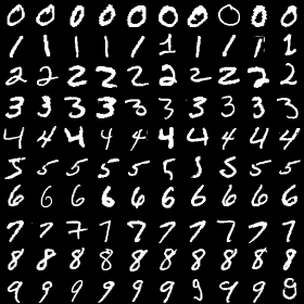
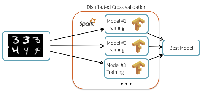
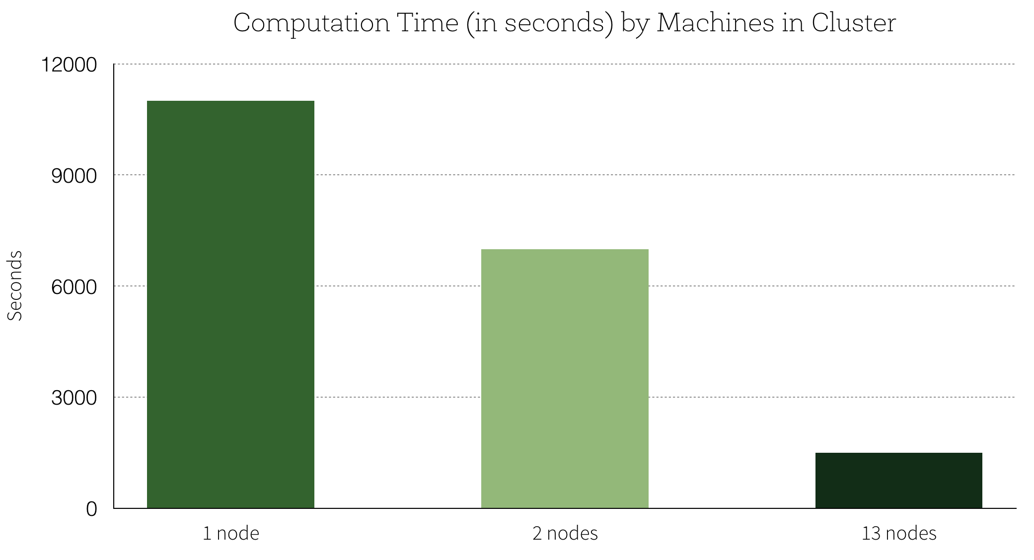
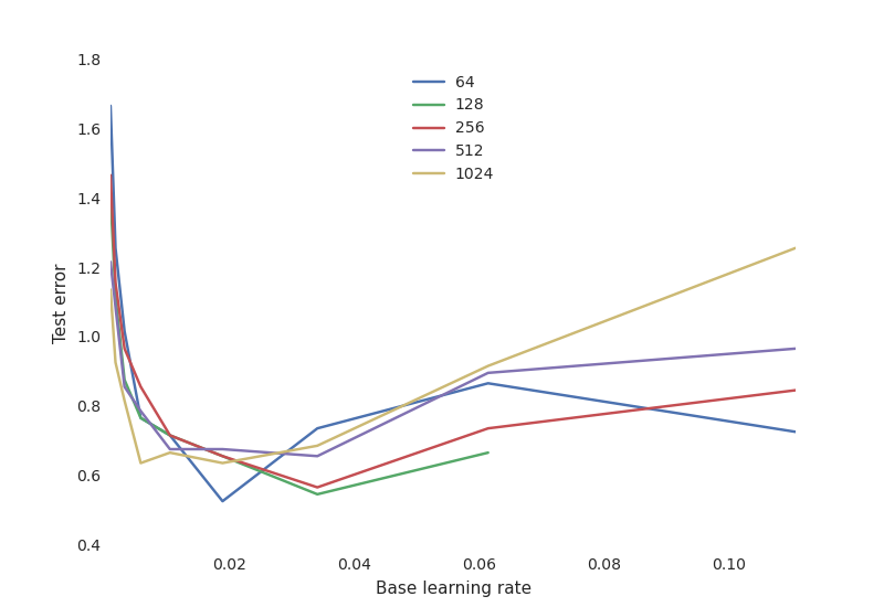


