http://www.pyimagesearch.com/2016/10/03/bubble-sheet-multiple-choice-scanner-and-test-grader-using-omr-python-and-opencv/
Over the past few months I’ve gotten quite the number of requests
landing in my inbox to build a bubble sheet/Scantron-like test reader
using computer vision and image processing techniques.
And while I’ve been having a lot of fun doing this series on machine learning and deep learning, I’d be
lying
if I said this little mini-project wasn’t a short, welcome break. One
of my favorite parts of running the PyImageSearch blog is demonstrating
how to build
actual solutions to problems using computer vision.
In fact, what makes this project
so special is that we are going to combine the techniques from
many previous blog posts, including
building a document scanner,
contour sorting, and
perspective transforms. Using
the knowledge gained from these previous posts, we’ll be able to make
quick work of this bubble sheet scanner and test grader.
You see, last Friday afternoon I quickly Photoshopped an example bubble test paper, printed out a few copies,
and then set to work on coding up the actual implementation.
Overall, I am quite pleased with this implementation and I think
you’ll absolutely be able to use this bubble sheet grader/OMR system as a
starting point for your own projects.
To learn more about utilizing computer vision, image processing, and OpenCV to automatically grade bubble test sheets, keep reading.
Bubble sheet scanner and test grader using OMR, Python, and OpenCV
In the remainder of this blog post, I’ll discuss what exactly
Optical Mark Recognition (OMR) is. I’ll then demonstrate how to implement a bubble sheet test scanner and grader using
strictly computer vision and image processing techniques, along with the OpenCV library.
Once we have our OMR system implemented, I’ll provide sample results
of our test grader on a few example exams, including ones that were
filled out with nefarious intent.
Finally, I’ll discuss some of the shortcomings of this current bubble
sheet scanner system and how we can improve it in future iterations.
What is Optical Mark Recognition (OMR)?
Optical Mark Recognition, or OMR for short, is the process of
automatically analyzing human-marked documents and interpreting their results.
Arguably, the most famous, easily recognizable form of OMR are
bubble sheet multiple choice tests, not unlike the ones you took in elementary school, middle school, or even high school.
If you’re unfamiliar with “bubble sheet tests” or the
trademark/corporate name of “Scantron tests”, they are simply
multiple-choice tests that you take as a student. Each question on the
exam is a multiple choice — and you use a #2 pencil to mark the “bubble”
that corresponds to the correct answer.
The most notable bubble sheet test you experienced (at least in the
United States) were taking the SATs during high school, prior to filling
out college admission applications.
I
believe that the SATs use the software provided by
Scantron to perform OMR and grade student exams, but I could easily be
wrong there. I only make note of this because Scantron is used in over
98% of all US school districts.
In short, what I’m trying to say is that there is a
massive market for Optical Mark Recognition and the ability to grade and interpret human-marked forms and exams.
Implementing a bubble sheet scanner and grader using OMR, Python, and OpenCV
Now that we understand the basics of OMR, let’s build a computer vision system using Python and OpenCV that can
read and
grade bubble sheet tests.
Of course, I’ll be providing lots of visual example images along the way so you can understand
exactly what techniques I’m applying and
why I’m using them.
Below I have included an example filled in bubble sheet exam that I have put together for this project:
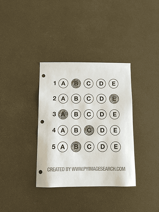
Figure 1: The example, filled in bubble sheet we are going to use when developing our test scanner software.
We’ll be using this as our example image as we work through the steps
of building our test grader. Later in this lesson, you’ll also find
additional sample exams.
I have also included a
blank exam template as a .PSD (Photoshop) file so you can modify it as you see fit. You can use the
“Downloads” section at the bottom of this post to download the code, example images, and template file.
The 7 steps to build a bubble sheet scanner and grader
The goal of this blog post is to build a bubble sheet scanner and test grader using Python and OpenCV.
To accomplish this, our implementation will need to satisfy the following 7 steps:
- Step #1: Detect the exam in an image.
- Step #2: Apply a perspective transform to extract the top-down, birds-eye-view of the exam.
- Step #3: Extract the set of bubbles (i.e., the possible answer choices) from the perspective transformed exam.
- Step #4: Sort the questions/bubbles into rows.
- Step #5: Determine the marked (i.e., “bubbled in”) answer for each row.
- Step #6: Lookup the correct answer in our answer key to determine if the user was correct in their choice.
- Step #7: Repeat for all questions in the exam.
The next section of this tutorial will cover the actual
implementation of our algorithm.
The bubble sheet scanner implementation with Python and OpenCV
To get started, open up a new file, name it
test_grader.py , and let’s get to work:
1
2
3
4
5
6
7
8
9
10
11
12
13
14
15
16
17
|
# import the necessary packages
from imutils.perspective import four_point_transform
from imutils import contours
import numpy as np
import argparse
import imutils
import cv2
# construct the argument parse and parse the arguments
ap = argparse.ArgumentParser()
ap.add_argument("-i", "--image", required=True,
help="path to the input image")
args = vars(ap.parse_args())
# define the answer key which maps the question number
# to the correct answer
ANSWER_KEY = {0: 1, 1: 4, 2: 0, 3: 3, 4: 1}
|
On
Lines 2-7 we import our required Python packages.
You should already have OpenCV and Numpy installed on your system, but you
might not have the most recent version of
imutils, my set of convenience functions to make performing basic image processing operations easier. To install
imutils (or upgrade to the latest version), just execute the following command:
|
|
$ pip install --upgrade imutils
|
Lines 10-12 parse our command line arguments. We only need a single switch here,
--image , which is the path to the input bubble sheet test image that we are going to grade for correctness.
Line 17 then defines our
ANSWER_KEY .
As the name of the variable suggests, the
ANSWER_KEY provides integer mappings of the
question numbers to the
index of the correct bubble.
In this case, a key of
0 indicates the
first question, while a value of
1 signifies
“B” as the correct answer (since
“B” is the index
1 in the string
“ABCDE”). As a second example, consider a key of
1 that maps to a value of
4 — this would indicate that the answer to the second question is
“E”.
As a matter of convenience, I have written the entire answer key in plain english here:
- Question #1: B
- Question #2: E
- Question #3: A
- Question #4: D
- Question #5: B
Next, let’s preprocess our input image:
|
|
# load the image, convert it to grayscale, blur it
# slightly, then find edges
image = cv2.imread(args["image"])
gray = cv2.cvtColor(image, cv2.COLOR_BGR2GRAY)
blurred = cv2.GaussianBlur(gray, (5, 5), 0)
edged = cv2.Canny(blurred, 75, 200)
|
On
Line 21 we load our image from disk, followed by converting it to grayscale (
Line 22), and blurring it to reduce high frequency noise (
Line 23).
We then apply the Canny edge detector on
Line 24 to find the
edges/outlines of the exam.
Below I have included a screenshot of our exam after applying edge detection:
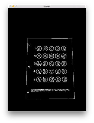
Figure 2: Applying edge detection to our exam neatly reveals the outlines of the paper.
Notice how the edges of the document are
clearly defined, with
all four vertices of the exam being present in the image.
Obtaining this silhouette of the document is
extremely important
in our next step as we will use it as a marker to apply a perspective
transform to the exam, obtaining a top-down, birds-eye-view of the
document:
26
27
28
29
30
31
32
33
34
35
36
37
38
39
40
41
42
43
44
45
46
47
48
49
|
# find contours in the edge map, then initialize
# the contour that corresponds to the document
cnts = cv2.findContours(edged.copy(), cv2.RETR_EXTERNAL,
cv2.CHAIN_APPROX_SIMPLE)
cnts = cnts[0] if imutils.is_cv2() else cnts[1]
docCnt = None
# ensure that at least one contour was found
if len(cnts) > 0:
# sort the contours according to their size in
# descending order
cnts = sorted(cnts, key=cv2.contourArea, reverse=True)
# loop over the sorted contours
for c in cnts:
# approximate the contour
peri = cv2.arcLength(c, True)
approx = cv2.approxPolyDP(c, 0.02 * peri, True)
# if our approximated contour has four points,
# then we can assume we have found the paper
if len(approx) == 4:
docCnt = approx
break
|
Now that we have the outline of our exam, we apply the
cv2.findContours function to find the lines that correspond to the exam itself.
We do this by sorting our contours by their
area (from largest to smallest) on
Line 37 (after making sure at least one contour was found on
Line 34,
of course). This implies that larger contours will be placed at the
front of the list, while smaller contours will appear farther back in
the list.
We make the assumption that our exam will be the
main focal point of the image,
and thus be larger than other objects in the image. This assumption
allows us to “filter” our contours, simply by investigating their area
and knowing that the contour that corresponds to the exam should be near
the front of the list.
However,
contour area and size is not enough — we should also check the number of
vertices on the contour.
To do, this, we loop over each of our (sorted) contours on
Line 40. For each of them, we approximate the contour, which in essence means we
simplify
the number of points in the contour, making it a “more basic” geometric
shape. You can read more about contour approximation in this post on
building a mobile document scanner.
On
Line 47 we make a check to see if our approximated contour has four points, and if it does,
we assume that we have found the exam.
Below I have included an example image that demonstrates the
docCnt variable being drawn on the original image:
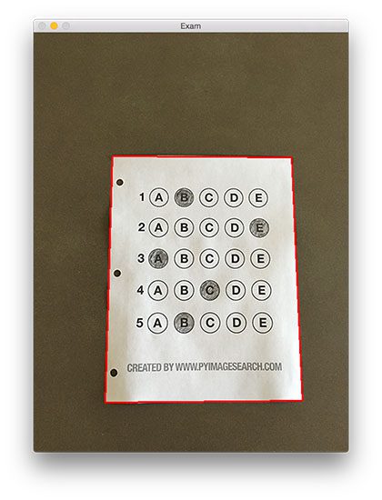
Figure 3:
An example of drawing the contour associated with the exam on our
original image, indicating that we have successfully found the exam.
Sure enough, this area corresponds to the outline of the exam.
Now that we have used contours to find the outline of the exam, we
can apply a perspective transform to obtain a top-down, birds-eye-view
of the document:
|
|
# apply a four point perspective transform to both the
# original image and grayscale image to obtain a top-down
# birds eye view of the paper
paper = four_point_transform(image, docCnt.reshape(4, 2))
warped = four_point_transform(gray, docCnt.reshape(4, 2))
|
In this case, we’ll be using my implementation of the
four_point_transform function which:
- Orders the (x, y)-coordinates of our contours in a specific, reproducible manner.
- Applies a perspective transform to the region.
You can learn more about the perspective transform in
this post as well as
this updated one on coordinate ordering,
but for the time being, simply understand that this function handles
taking the “skewed” exam and transforms it, returning a top-down view of
the document:
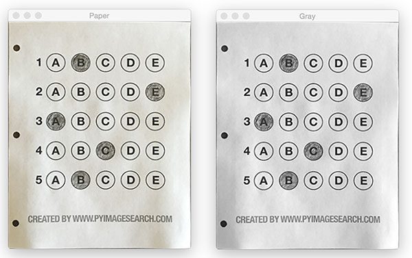
Figure 4: Obtaining a top-down, birds-eye view of both the original image (left) along with the grayscale version (right).
Alright, so now we’re getting somewhere.
We found our exam in the original image.
We applied a perspective transform to obtain a 90 degree viewing angle of the document.
But how do we go about actually
grading the document?
This step starts with
binarization, or the process of thresholding/segmenting the
foreground from the
background of the image:
|
|
# apply Otsu's thresholding method to binarize the warped
# piece of paper
thresh = cv2.threshold(warped, 0, 255,
cv2.THRESH_BINARY_INV | cv2.THRESH_OTSU)[1]
|
After applying Otsu’s thresholding method, our exam is now a
binary image:
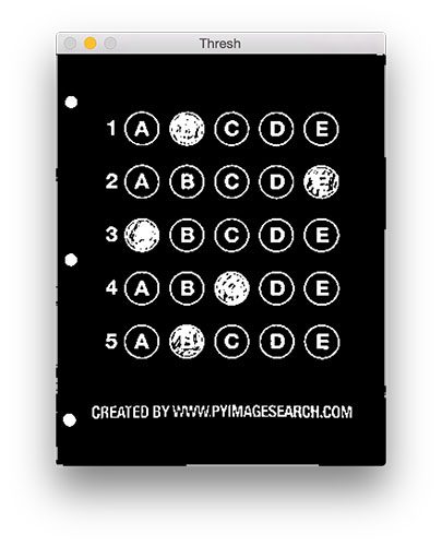
Figure 5: Using Otsu’s thresholding allows us to segment the foreground from the background of the image.
Notice how the
background of the image is
black, while the
foreground is
white.
This binarization will allow us to once again apply contour extraction techniques to find each of the bubbles in the exam:
62
63
64
65
66
67
68
69
70
71
72
73
74
75
76
77
78
79
80
|
# find contours in the thresholded image, then initialize
# the list of contours that correspond to questions
cnts = cv2.findContours(thresh.copy(), cv2.RETR_EXTERNAL,
cv2.CHAIN_APPROX_SIMPLE)
cnts = cnts[0] if imutils.is_cv2() else cnts[1]
questionCnts = []
# loop over the contours
for c in cnts:
# compute the bounding box of the contour, then use the
# bounding box to derive the aspect ratio
(x, y, w, h) = cv2.boundingRect(c)
ar = w / float(h)
# in order to label the contour as a question, region
# should be sufficiently wide, sufficiently tall, and
# have an aspect ratio approximately equal to 1
if w >= 20 and h >= 20 and ar >= 0.9 and ar <= 1.1:
questionCnts.append(c)
|
Lines 64-67 handle finding contours on our
thresh binary image, followed by initializing
questionCnts , a list of contours that correspond to the questions/bubbles on the exam.
To determine which regions of the image are bubbles, we first loop over each of the individual contours (
Line 70).
For each of these contours, we compute the bounding box (
Line 73), which also allows us to compute the
aspect ratio, or more simply, the ratio of the width to the height (
Line 74).
In order for a contour area to be considered a bubble, the region should:
- Be sufficiently wide and tall (in this case, at least 20 pixels in both dimensions).
- Have an aspect ratio that is approximately equal to 1.
As long as these checks hold, we can update our
questionCnts list and mark the region as a bubble.
Below I have included a screenshot that has drawn the output of
questionCnts on our image:
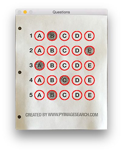
Figure 6: Using contour filtering allows us to find all the question bubbles in our bubble sheet exam recognition software.
Notice how
only the question regions of the exam are highlighted and nothing else.
We can now move on to the “grading” portion of our OMR system:
82
83
84
85
86
87
88
89
90
91
92
93
94
95
|
# sort the question contours top-to-bottom, then initialize
# the total number of correct answers
questionCnts = contours.sort_contours(questionCnts,
method="top-to-bottom")[0]
correct = 0
# each question has 5 possible answers, to loop over the
# question in batches of 5
for (q, i) in enumerate(np.arange(0, len(questionCnts), 5)):
# sort the contours for the current question from
# left to right, then initialize the index of the
# bubbled answer
cnts = contours.sort_contours(questionCnts[i:i + 5])[0]
bubbled = None
|
First, we must sort our
questionCnts from top-to-bottom. This will ensure that rows of questions that are
closer to the top of the exam will appear
first in the sorted list.
We also initialize a bookkeeper variable to keep track of the number of
correct answers.
On
Line 90 we start looping over our questions.
Since each question has 5 possible answers, we’ll apply NumPy array
slicing and contour sorting to to sort the
current set of contours from left to right.
The reason this methodology works is because we have
already sorted our contours from top-to-bottom. We
know that the 5 bubbles for each question will appear sequentially in our list —
but we do not know whether these bubbles will be sorted from left-to-right. The sort contour call on
Line 94 takes care of this issue and ensures each row of contours are sorted into rows, from left-to-right.
To visualize this concept, I have included a screenshot below that depicts each row of questions as a separate color:
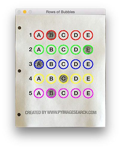
Figure 7:
By sorting our contours from top-to-bottom, followed by left-to-right,
we can extract each row of bubbles. Therefore, each row is equal to the
bubbles for one question.
Given a row of bubbles, the next step is to determine which bubble is filled in.
We can accomplish this by using our
thresh image and counting the number of non-zero pixels (i.e.,
foreground pixels) in each bubble region:
97
98
99
100
101
102
103
104
105
106
107
108
109
110
111
112
113
114
|
# loop over the sorted contours
for (j, c) in enumerate(cnts):
# construct a mask that reveals only the current
# "bubble" for the question
mask = np.zeros(thresh.shape, dtype="uint8")
cv2.drawContours(mask, [c], -1, 255, -1)
# apply the mask to the thresholded image, then
# count the number of non-zero pixels in the
# bubble area
mask = cv2.bitwise_and(thresh, thresh, mask=mask)
total = cv2.countNonZero(mask)
# if the current total has a larger number of total
# non-zero pixels, then we are examining the currently
# bubbled-in answer
if bubbled is None or total > bubbled[0]:
bubbled = (total, j)
|
Line 98 handles looping over each of the sorted bubbles in the row.
We then construct a mask for the current bubble on
Line 101 and then count the number of non-zero pixels in the masked region (
Lines 107 and 108).
The more non-zero pixels we count, then the more foreground pixels
there are, and therefore the bubble with the maximum non-zero count is
the index of the bubble that the the test taker has bubbled in (
Line 113 and 114).
Below I have included an example of creating and applying a mask to each bubble associated with a question:
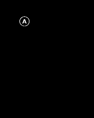
Figure 8: An example of constructing a mask for each bubble in a row.
Clearly, the bubble associated with
“B” has the most thresholded pixels, and is therefore the bubble that the user has marked on their exam.
This next code block handles looking up the correct answer in the
ANSWER_KEY , updating any relevant bookkeeper variables, and finally drawing the marked bubble on our image:
116
117
118
119
120
121
122
123
124
125
126
127
|
# initialize the contour color and the index of the
# *correct* answer
color = (0, 0, 255)
k = ANSWER_KEY[q]
# check to see if the bubbled answer is correct
if k == bubbled[1]:
color = (0, 255, 0)
correct += 1
# draw the outline of the correct answer on the test
cv2.drawContours(paper, [cnts[k]], -1, color, 3)
|
Based on whether the test taker was correct or incorrect yields which color is drawn on the exam. If the test taker is
correct, we’ll highlight their answer in
green. However, if the test taker made a mistake and marked an incorrect answer, we’ll let them know by highlighting the
correct answer in
red:
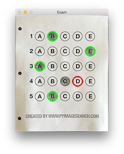
Figure 9: Drawing a “green” circle to mark “correct” or a “red” circle to mark “incorrect”.
Finally, our last code block handles scoring the exam and displaying the results to our screen:
129
130
131
132
133
134
135
136
|
# grab the test taker
score = (correct / 5.0) * 100
print("[INFO] score: {:.2f}%".format(score))
cv2.putText(paper, "{:.2f}%".format(score), (10, 30),
cv2.FONT_HERSHEY_SIMPLEX, 0.9, (0, 0, 255), 2)
cv2.imshow("Original", image)
cv2.imshow("Exam", paper)
cv2.waitKey(0)
|
Below you can see the output of our fully graded example image:
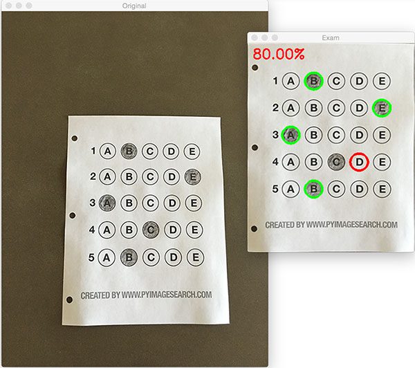
Figure 10: Finishing our OMR system for grading human-taken exams.
In this case, the reader obtained an 80% on the exam. The only question they missed was #4 where they incorrectly marked
“C” as the correct answer (
“D” was the correct choice).
Why not use circle detection?
After going through this tutorial, you might be wondering:
“Hey Adrian, an answer bubble is a circle. So why did you extract contours instead of applying Hough circles to find the circles in the image?”
Great question.
To start, tuning the parameters to Hough circles on an image-to-image basis can be a real pain. But that’s only a minor reason.
The
real reason is:
User error.
How many times, whether purposely or not, have you filled in outside
the lines on your bubble sheet? I’m not expert, but I’d have to guess
that at least 1 in every 20 marks a test taker fills in is “slightly”
outside the lines.
And guess what?
Hough circles don’t handle deformations in their outlines very well — your circle detection would totally fail in that case.
Because of this, I instead recommend using contours and contour properties to help you filter the bubbles and answers. The
cv2.findContours function doesn’t care if the bubble is “round”, “perfectly round”, or “oh my god, what the hell is that?”.
Instead, the
cv2.findContours function will return a set of
blobs
to you, which will be the foreground regions in your image. You can
then take these regions process and filter them to find your questions
(as we did in this tutorial), and go about your way.
Our bubble sheet test scanner and grader results
To see our bubble sheet test grader in action, be sure to download the source code and example images to this post using the
“Downloads” section at the bottom of the tutorial.
We’ve already seen
test_01.png as our example earlier in this post, so let’s try
test_02.png :
|
|
$ python test_grader.py --image images/test_02.png
|
Here we can see that a particularly nefarious user took our exam. They were not happy with the test, writing
“#yourtestsux” across the front of it along with an anarchy inspiring
“#breakthesystem”. They also marked
“A” for all answers.
Perhaps it comes as no surprise that the user scored a pitiful 20% on the exam, based entirely on luck:
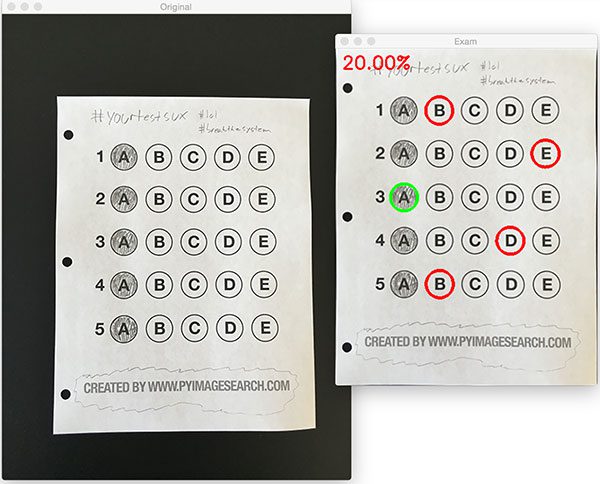
Figure 11: By using contour filtering, we are able to ignore the regions of the exam that would have otherwise compromised its integrity.
Let’s try another image:
|
|
$ python test_grader.py --image images/test_03.png
|
This time the reader did a little better, scoring a 60%:
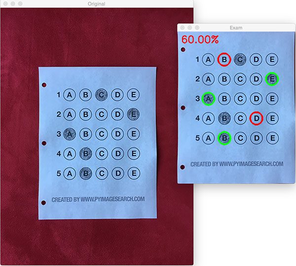
Figure 12: Building a bubble sheet scanner and test grader using Python and OpenCV.
In this particular example, the reader simply marked all answers along a diagonal:
|
|
$ python test_grader.py --image images/test_04.png
|
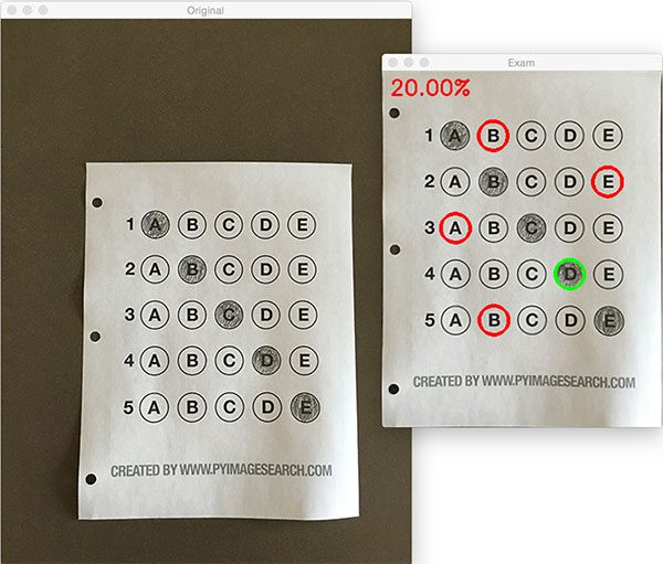
Figure 13: Optical Mark Recognition for test scoring using Python and OpenCV.
Unfortunately for the test taker, this strategy didn’t pay off very well.
Let’s look at one final example:
|
|
$ python test_grader.py --image images/test_05.png
|
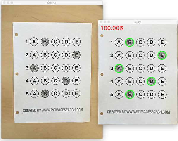
Figure 14: Recognizing bubble sheet exams using computer vision.
This student clearly studied ahead of time, earning a perfect 100% on the exam.
Extending the OMR and test scanner
Admittedly, this past summer/early autumn has been one of the
busiest periods of my life, so I needed to
timebox the development of the OMR and test scanner software into a single, shortened afternoon last Friday.
While I was able to get the barebones of a
working bubble
sheet test scanner implemented, there are certainly a few areas that
need improvement. The most obvious area for improvement is the
logic to handle non-filled in bubbles.
In the current implementation, we (naively) assume that a reader has filled in
one and
only one bubble per question row.
However, since we determine if a particular bubble is “filled in”
simply by counting the number of thresholded pixels in a row and then
sorting in descending order, this can lead to two problems:
- What happens if a user does not bubble in an answer for a particular question?
- What if the user is nefarious and marks multiple bubbles as “correct” in the same row?
Luckily, detecting and handling of these issues isn’t terribly challenging, we just need to insert a bit of logic.
For issue #1, if a reader chooses
not to bubble in an answer for a particular row, then we can place a
minimum threshold on
Line 108 where we compute
cv2.countNonZero :
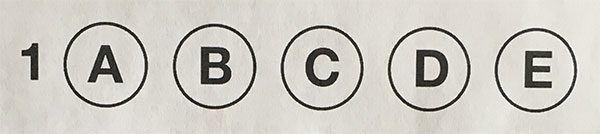
Figure 15: Detecting if a user has marked zero bubbles on the exam.
If this value is sufficiently large, then we can mark the bubble as “filled in”. Conversely, if
total is too small, then we can skip that particular bubble. If at the end of the row there are
no bubbles with sufficiently large threshold counts, we can mark the question as “skipped” by the test taker.
A similar set of steps can be applied to issue #2, where a user marks
multiple bubbles as correct for a single question:
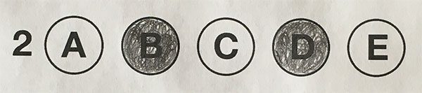
Figure 16: Detecting if a user has marked multiple bubbles for a given question.
Again, all we need to do is apply our thresholding and count step, this time keeping track if there are
multiple bubbles that have a
total that exceeds some pre-defined value. If so, we can invalidate the question and mark the question as incorrect.
Summary
In this blog post, I demonstrated how to build a bubble sheet scanner
and test grader using computer vision and image processing techniques.
Specifically, we implemented
Optical Mark Recognition (OMR) methods that facilitated our ability of capturing human-marked documents and
automatically analyzing the results.
Finally, I provided a Python and OpenCV implementation that you can use for building your own bubble sheet test grading systems.
If you have any questions, please feel free to leave a comment in the comments section!
But before you, be sure to enter your email address in
the form below to be notified when future tutorials are published on the
PyImageSearch blog!