This
post is meant to constitute an intuitive explanation of the SSD
MultiBox object detection technique. I have tried to minimise the maths
and instead slowly guide you through the tenets of this architecture,
which includes explaining what the MultiBox algorithm does. After
reading this post, I hope you will have a better grasp of SSD and will
try it out for yourselves!
Since AlexNet
took the research world by storm at the 2012 ImageNet Large-Scale
Visual Recognition Challenge (ILSVRC), deep learning has become the
go-to method for image recognition tasks, far surpassing more
traditional computer vision methods used in the literature. In the field
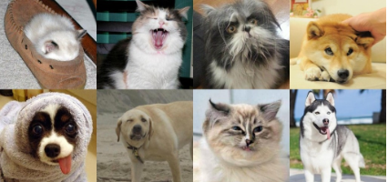
of computer vision, convolution neural networks excel at image classification, which consists of categorising images, given a set of classes (e.g. cat, dog), and having the network determine the strongest class present in the image.
Images of cats and dogs (from kaggle)
Nowadays,
deep learning networks are better at image classification than humans,
which shows just how powerful this technique is. However, we as humans
do far more than just classify images when observing and interacting
with the world. We also localize and classify
each element within our field of view. These are much more complex
tasks which machines are still struggling to perform as well as humans.
In fact, I would argue that object detection when performed well, brings
machines closer to real scene understanding.
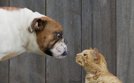
Does the image show cat, a dog, or do we have both? (from kaggle)
The Region-Convolutional Neural Network (R-CNN)
A
few years ago, by exploiting some of the leaps made possible in
computer vision via CNNs, researchers developed R-CNNs to deal with the
tasks of object detection, localization and classification. Broadly
speaking, a R-CNN is a special type of CNN that is able to locate and
detect objects in images: the output is generally a set of bounding
boxes that closely match each of the detected objects, as well as a
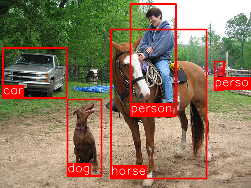
class output for each detected object. The image below shows what a
typical R-CNN outputs:
Example output of R-CNN
There
is an exhaustive list of papers in this field and for anyone eager to
explore further I recommend starting with the following “trilogy” of
papers around the topic:
As
you might have guessed, each next paper proposes improvements to the
seminal work done in R-CNN to develop a faster network, with the goal of
achieving real-time object detection. The achievements displayed
through this set of work is truly amazing, yet none of these
architectures manage to create a real-time object detector. Without
going too much into details, the following problems with the above
networks were identified:
Training the data is unwieldy and too long
Training happens in multiple phases (e.g. training region proposal vs classifier)
Network is too slow at inferencetime (i.e. when dealing with non-training data)
Fortunately,
in the last few years, new architectures were created to address the
bottlenecks of R-CNN and its successors, enabling real-time object
detection. The most famous ones are YOLO (You Only Look Once) and SSD
MultiBox (Single Shot Detector). In this post, we will discuss SSD as
there seem to be less coverage about this architecture than YOLO.
Besides, you should also find it easier to grasp YOLO once you
understand SSD.
Single Shot MultiBox Detector
The paper about SSD: Single Shot MultiBox Detector
(by C. Szegedy et al.) was released at the end of November 2016 and
reached new records in terms of performance and precision for object
detection tasks, scoring over 74% mAP (meanAverage Precision) at 59 frames per second on standard datasets such as PascalVOC and COCO. To better understand SSD, let’s start by explaining where the name of this architecture comes from:
Single Shot: this means that the tasks of object localization and classificationare done in a singleforward pass of the network
MultiBox: this is the name of a technique for bounding box regression developed by Szegedy et al. (we will briefly cover it shortly)
Detector: The network is an object detector that also classifies those detected objects
Architecture
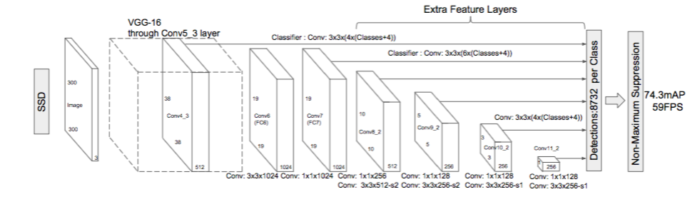
Architecture of Single Shot MultiBox detector (input is 300x300x3)
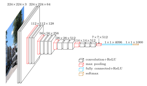
As
you can see from the diagram above, SSD’s architecture builds on the
venerable VGG-16 architecture, but discards the fully connected layers.
The reason VGG-16 was used as the base network is because of its strong performance in high quality image classification tasks and its popularity for problems where transfer learning helps in improving results. Instead of the original VGG fully connected layers, a set of auxiliary convolutional layers (from conv6 onwards)
were added, thus enabling to extract features at multiple scales and
progressively decrease the size of the input to each subsequent layer.
VGG architecture (input is 224x224x3)
MultiBox
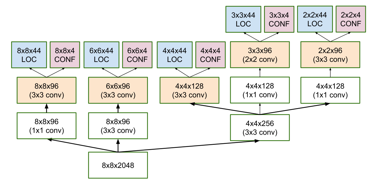
The bounding box regression technique of SSD is inspired by Szegedy’s work on MultiBox, a method for fast class-agnostic bounding box coordinate proposals. Interestingly, in the work done on MultiBox an Inception-style
convolutional network is used. The 1x1 convolutions that you see below
help in dimensionality reduction since the number of dimensions will go
down (but “width” and “height” will remain the same).
Architecture of multi-scale convolutional prediction of the location and confidences of multibox
MultiBox’s loss function also combined two critical components that made their way into SSD:
Confidence Loss: this measures how confident the network is of the objectness of the computed bounding box. Categorical cross-entropy is used to compute this loss.
Location Loss: this measures how far away the network’s predicted bounding boxes are from the ground truth ones from the training set. L2-Norm is used here.
Without
delving too deep into the math (read the paper if you are curious and
want a more rigorous notation), the expression for the loss, which
measures how far off our prediction “landed”, is thus:
The alpha term
helps us in balancing the contribution of the location loss. As usual
in deep learning, the goal is to find the parameter values that most
optimally reduce the loss function, thereby bringing our predictions
closer to the ground truth.
MultiBox Priors And IoU
The
logic revolving around the bounding box generation is actually more
complex than what I earlier stated. But fear not: it is still within
reach.
In MultiBox, the researchers created what we call priors (or anchors in
Faster-R-CNN terminology), which are pre-computed, fixed size bounding
boxes that closely match the distribution of the original ground truth
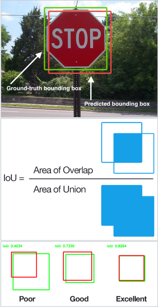
boxes. In fact those priors are selected in such a way that their Intersection over Union ratio (aka IoU, and sometimes referred to as Jaccard index)
is greater than 0.5. As you can infer from the image below, an IoU of
0.5 is still not good enough but it does however provide a strong
starting point for the bounding box regression algorithm — it is a much
better strategy than starting the predictions with random coordinates! Therefore MultiBox starts with the priors as predictions and attempt to regress closer to the ground truth bounding boxes.
Diagram explaining IoU (from Wikipedia)
The
resulting architecture (check MultiBox architecture diagram above again
for reference) contains 11 priors per feature map cell (8x8, 6x6, 4x4,
3x3, 2x2) and only one on the 1x1 feature map, resulting in a total of
1420 priors per image, thus enabling robust coverage of input images at
multiple scales, to detect objects of various sizes.
At the end, MultiBox only retains the top K predictions that have minimised both location (LOC) and confidence (CONF) losses.
SSD Improvements
Back onto SSD, a number of tweaks were added to make this network even more capable of localizing and classifying objects.
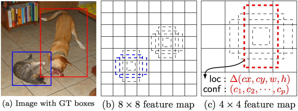
Fixed Priors: unlike
MultiBox, every feature map cell is associated with a set of default
bounding boxes of different dimensions and aspect ratios. These priors
are manually (but carefully) chosen, whereas in MultiBox, they were
chosen because their IoU with respect to the ground truth was over 0.5.
This in theory should allow SSD to generalise for any type of input,
without requiring a pre-training phase for prior generation. For
instance, assuming we have configured b defaultbounding boxes per feature map cell, and c classes to classify, on a given feature map of size f =m x n, SSD would compute f(b + c) values for this feature map.
SSD default boxes at 8x8 and 4x4 feature maps
Location Loss: SSDuses smooth L1-Norm
to calculate the location loss. While not as precise as L2-Norm, it is
still highly effective and gives SSD more room for manoeuvre as it does
not try to be “pixel perfect” in its bounding box prediction (i.e. a
difference of a few pixels would hardly be noticeable for many of us).
Classification: MultiBox does not perform object classification, whereas SSD does. Therefore, for each predicted bounding box, a set of c class predictions are computed, for every possible class in the dataset.
Training & Running SSD
Datasets
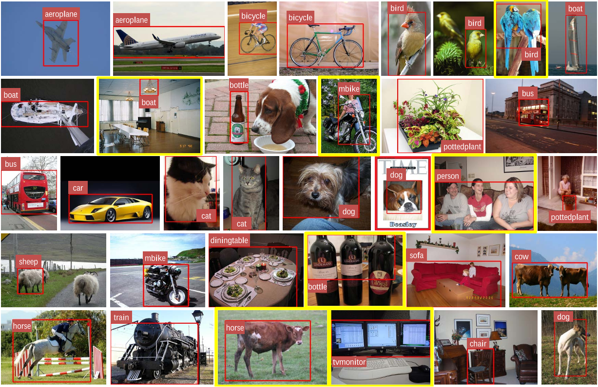
You
will need training and test datasets with ground truth bounding boxes
and assigned class labels (only one per bounding box). The Pascal VOC
and COCO datasets are a good starting point.
Images from Pascal VOC dataset
Default Bounding Boxes
It
is recommended to configure a varied set of default bounding boxes, of
different scales and aspect ratios to ensure most objects could be
captured. The SSD paper has around 6 bounding boxes per feature map
cell.
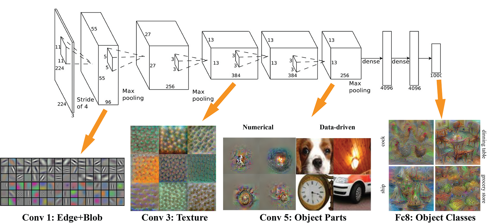
Feature Maps
Features
maps (i.e. the results of the convolutional blocks) are a
representation of the dominant features of the image at different
scales, therefore running MultiBox on multiple feature maps increases
the likelihood of any object (large and small) to be eventually
detected, localized and appropriately classified. The image below shows
how the network “sees” a given image across its feature maps:
VGG Feature Map Visualisation (from Brown Uni)
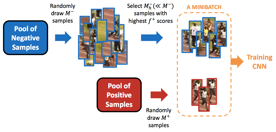
Hard Negative Mining
During training, as most of the bounding boxes will have low IoU and therefore be interpreted as negative training
examples, we may end up with a disproportionate amount of negative
examples in our training set. Therefore, instead of using all negative
predictions, it is advised to keep a ratio of negative to positive
examples of around 3:1. The reason why you need to keep negative samples
is because the network also needs to learn and be explicitly told what
constitutes an incorrect detection.
Example of hard negative mining (from Jamie Kang blog)
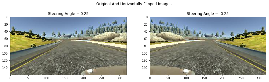
Data Augmentation
The
authors of SSD stated that data augmentation, like in many other deep
learning applications, has been crucial to teach the network to become
more robust to various object sizes in the input. To this end, they
generated additional training examples with patches of the original
image at different IoU ratios (e.g. 0.1, 0.3, 0.5, etc.) and random
patches as well. Moreover, each image is also randomly horizontally
flipped with a probability of 0.5, thereby making sure potential objects
appear on left and right with similar likelihood.
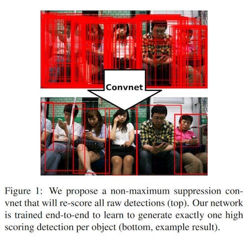
Given
the large number of boxes generated during a forward pass of SSD at
inference time , it is essential to prune most of the bounding box by
applying a technique known as non-maximum suppression: boxes with a confidence loss threshold less than ct (e.g. 0.01) and IoU less than lt (e.g. 0.45) are discarded, and only the top N predictions
are kept. This ensures only the most likely predictions are retained by
the network, while the more noisier ones are removed.
The SSD paper makes the following additional observations:
more default boxes results in more accurate detection, although there is an impact on speed
having
MultiBox on multiple layers results in better detection as well, due to
the detector running on features at multiple resolutions
80%
of the time is spent on the base VGG-16 network: this means that with a
faster and equally accurate network SSD’s performance could be even
better
SSD confuses objects with similar categories (e.g. animals). This is probably because locations are shared for multiple classes
SSD-500
(the highest resolution variant using 512x512 input images) achieves
best mAP on Pascal VOC2007 at 76.8%, but at the expense of speed, where
its frame rate drops to 22 fps. SSD-300 is thus a much better trade-off
with 74.3 mAP at 59 fps.
SSD
produces worse performance on smaller objects, as they may not appear
across all feature maps. Increasing the input image resolution
alleviates this problem but does not completely address it
Playing With SSD
There are a few implementations of SSD available online, including the original Caffe code from the authors of the paper. In my case, I opted for Paul Balança’s TensorFlow implementation, available on github. It is worth reading the code as well the paper to better understand how everything fits together.
I also recently decided to reimplement a project on Vehicle Detection
that was using traditional computer vision techniques, by employing SSD
this time. A small gif of my output using SSD shows it works very well:
GIF of vehicle detection Using SSD
Beyond SSD
More
recent work in this field has been produced, and I would recommend
following up on the two papers below for anyone interested in pushing
their knowledge further in this domain:
Mask R-CNN: very accurate instance segmentation at pixel level
Voilà!
We are done with our tour of Single Shot MultiBox Detector. I tried to
explain the concepts behind this technique in simple terms, as best as I
understood them, with many pictures to further illustrate those
concepts and facilitate your understanding. I do really recommend
reading the paper (probably a few times if you are slow like me 🙃),
including forming good intuition behind some of the maths in this
technique to cement your comprehension. You can always check this post
if some of its sections help you make sense of the paper. Godspeed!
The goal of this website is to provide a testbed for developing new VLBI reconstruction algorithms.
By supplying a large set of easy to understand training and testing data, we hope to make the problem more accessible to those
less familiar with the VLBI field. Specifically, this website contains a:
Online form to easily simulate realistic data using your own image and telescope parameters
What is VLBI Imaging?
Imaging distant celestial sources with high resolving
power requires telescopes with prohibitively large diameters due to the
inverse relationship between angular resolution and telescope diameter.
However, by simultaneously collecting data from an array of telescopes
located around the Earth, it is possible to emulate samples from a
single telescope with a diameter equal to the maximum distance between
telescopes in the array. Using multiple telescopes in this manner is
referred to as very long baseline interferometry (VLBI). Reconstructing an image using VLBI measurements is
an ill-posed problem, and as such each there are an infinite number of
possible images that explain the data. The challenge is to find an
explanation that respects these prior assumptions while still satisfying
the observed data. The goal of this website to aid in the process of
developing these algorithms as well as evaluate their performance.
The ongoing international effort to create an
Event Horizon Telescope
capable of imaging the enviroment around a black
hole’s event horizon calls for the use of VLBI
reconstruction algorithms. The angular resolution necessary for these
measurements requires overcoming
many challenges, all of which make image
reconstruction
more difficult.
For instance, at the mm/sub-mm wavelengths being
observed,
rapidly varying inhomogeneities in the atmosphere
introduce
additional measurement errors.
Robust algorithms that are able to reconstruct
images
in this fine angular resolution regime are essential
for scientific progress.
The spectacular recent successes of deep learning are purely empirical.
Nevertheless intellectuals always try to explain important developments
theoretically. In this literature course we will review recent work of
Bruna and Mallat, Mhaskar and Poggio, Papyan and Elad, Bolcskei and
co-authors, Baraniuk and co-authors, and others, seeking to build
theoretical frameworks deriving deep networks as consequences. After
initial background lectures, we will have some of the authors presenting
lectures on specific papers. This course meets once weekly.
Over
the past few months, I have been collecting AI cheat sheets. From time
to time I share them with friends and colleagues and recently I have
been getting asked a lot, so I decided to organize and share the entire
collection. To make things more interesting and give context, I added
descriptions and/or excerpts for each major topic.
This is the most complete list and the Big-O is at the very end, enjoy…