
Friday, May 27, 2016
Sunday, May 15, 2016
Setting up a Deep Learning Machine from Scratch
https://github.com/saiprashanths/dl-setup
There are several great guides with a similar goal. Some are limited in scope, while others are not up to date. This guide is based on (with some portions copied verbatim from):
Setting up a Deep Learning Machine from Scratch (Software)
A detailed guide to setting up your machine for deep learning research. Includes instructions to install drivers, tools and various deep learning frameworks. This was tested on a 64 bit machine with Nvidia Titan X, running Ubuntu 14.04There are several great guides with a similar goal. Some are limited in scope, while others are not up to date. This guide is based on (with some portions copied verbatim from):
Table of Contents
Basics
Sunday, May 8, 2016
Number plate recognition with Tensorflow
https://matthewearl.github.io/2016/05/06/cnn-anpr/
In order to get some hands-on experience with implementing neural networks I decided I’d design a system to solve a similar problem: Automated number plate recognition (automated license plate recognition if you’re in the US). My reasons for doing this are three-fold:
128x64 was chosen as the input resolution as this is small enough to permit training in a reasonable amount of time with modest resources, but also large enough for number plates to be somewhat readable:
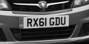
Image credit
In order to detect number plates in larger images a sliding window approach is used at various scales:
Image credit
The image on the right is the 128x64 input that the neural net sees, whereas the left shows the window in the context of the original input image.
For each window the network should output:
2‾√
times between zoom levels and be guaranteed not to miss any plates, while at the same time not generating an excessive number of matches for any single plate. Any duplicates that do occur are combined in a post-processing step (explained later).
The process for generating the images is illustrated below:

The text and plate colour are chosen randomly, but the text must be a certain amount darker than the plate. This is to simulate real-world lighting variation. Noise is added at the end not only to account for actual sensor noise, but also to avoid the network depending too much on sharply defined edges as would be seen with an out-of-focus input image.
Having a background is important as it means the network must learn to identify the bounds of the number plate without “cheating”: Were a black background used for example, the network may learn to identify plate location based on non-blackness, which would clearly not work with real pictures of cars.
The backgrounds are sourced from the SUN database, which contains over 100,000 images. It’s important the number of images is large to avoid the network “memorizing” background images.
The transformation applied to the plate (and its mask) is an affine transformation based on a random roll, pitch, yaw, translation, and scale. The range allowed for each parameter was selected according to the ranges that number plates are likely to be seen. For example, yaw is allowed to vary a lot more than roll (you’re more likely to see a car turning a corner, than on its side).
The code to generate the images is relatively short (~300 lines). It can be read in gen.py.

See the wikipedia page for a summary of CNN building blocks. The above network is in fact based on this paper by Stark et al, as it gives more specifics about the architecture used than the Google paper.
The output layer has one node (shown on the left) which is used as the presence indicator. The rest encode the probability of a particular number plate: Each column as shown in the diagram corresponds with one of the digits in the number plate, and each node gives the probability of the corresponding character being present. For example, the node in column 2 row 3 gives the probability that the second digit is a
As is standard with deep neural nets all but the output layers use ReLU activation. The presence node has sigmoid activation as is typically used for binary outputs. The other output nodes use softmax across characters (ie. so that the probability in each column sums to one) which is the standard approach for modelling discrete probability distributions.
The code defining the network is in model.py.
The loss function is defined in terms of the cross-entropy between the label and the network output. For numerical stability the activation functions of the final layer are rolled into the cross-entropy calculation using
Training (train.py) takes about 6 hours using a nVidia GTX 970, with training data being generated on-the-fly by a background process on the CPU.
The network differs from the one used in training in that the last two layers are convolutional rather than fully connected, and the input image can be any size rather than 128x64. The idea is that the whole image at a particular scale can be fed into this network which yields an image with a presence / character probability values at each “pixel”. The idea here is that adjacent windows will share many convolutional features, so rolling them into the same network avoids calculating the same features multiple times.
Visualizing the “presence” portion of the output yields something like the following:
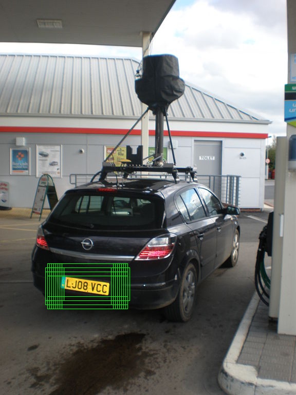
Image credit
The boxes here are regions where the network detects a greater than 99% probability that a number plate is present. The reason for the high threshold is to account for a bias introduced in training: About half of the training images contained a number plate, whereas in real world images of cars number plates are much rarer. As such if a 50% threshold is used the detector is prone to false positives.
To cope with the obvious duplicates we apply a form of non-maximum suppression to the output:
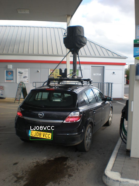
Image credit
The technique used here first groups the rectangles into overlapping rectangles, and for each group outputs:
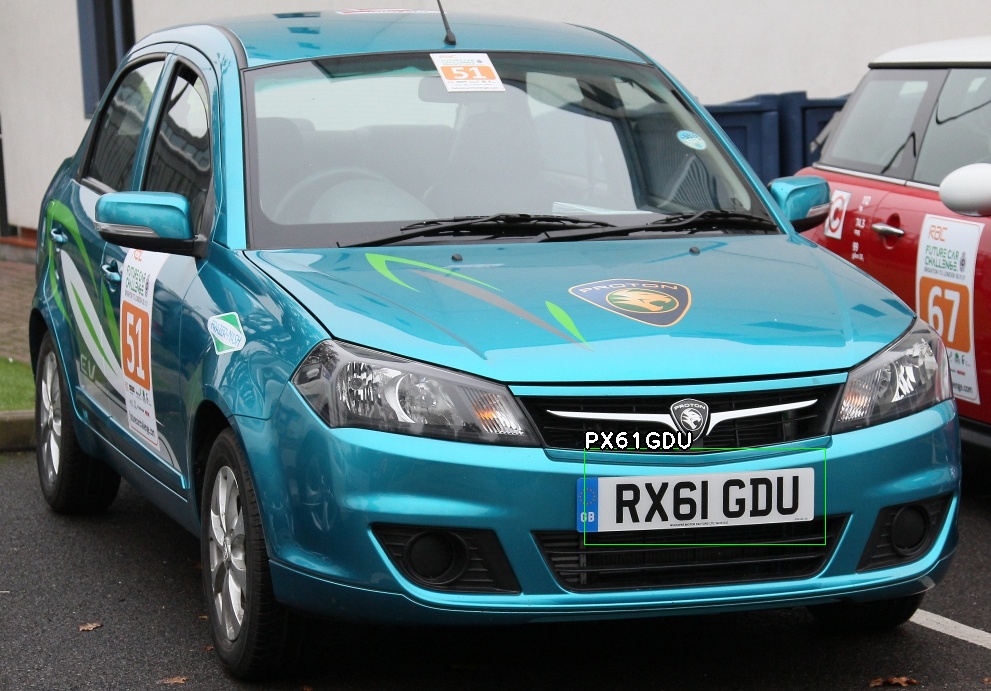
Image credit
Whoops, the R has been misread as a P. Here’s the window from the above image which gives the maximum presence response:
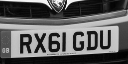
Image credit
On first glance it appears that this should be an easy case for the detector, however it turns out to be an instance of overfitting. Here’s the R from the number plate font used to generate the training images:

Note how the leg of the R is at a different angle to the leg of the R in the input image. The network has only ever seen R’s as shown above, so gets confused when it sees R’s in a different font. To test this hypothesis I modified the image in GIMP to more closely resemble the training font:
And sure enough, the detector now gets the correct result:

The code for the detector is in detect.py.
On the other hand, my system has a number of drawbacks:
I showed an instance of 2) above, with the misdetection of an R due to a slightly varied font. The effects would be further exacerbated if I were trying to detect US number plates rather than UK number plates which have much more varied fonts. One possible solution would be to make my training data more varied by drawing from a selection of fonts, although it’s not clear how many fonts I would need for this approach to be successful.
The slowness (3)) is a killer for many applications: A modestly sized input image takes a few seconds to process on a reasonably powerful GPU. I don’t think its possible to get away from this without introducing a (cascade of) detection stages, for example a Haar cascade, a HOG detector, or a simpler neural net.
It would be an interesting exercise to see how other ML techniques compare, in particular pose regression (with the pose being an affine transformation corresponding with 3 corners of the plate) looks promising. A much more basic classification stage could then be tacked on the end. This solution should be similarly terse if an ML library such as scikit-learn is used.
In conclusion, I’ve shown that a single CNN (with some filtering) can be used as a passable number plate detector / recognizer, however it does not yet compete with the traditional hand-crafted (but more verbose) pipelines in terms of performance.
Original “Google Street View Car” image by Reedy licensed under the Creative Commons Attribution-Share Alike 3.0 Unported license.
Introduction
Over the past few weeks I’ve been dabbling with deep learning, in particular convolutional neural networks. One standout paper from recent times is Google’s Multi-digit Number Recognition from Street View. This paper describes a system for extracting house numbers from street view imagery using a single end-to-end neural network. The authors then go on to explain how the same network can be applied to breaking Google’s own CAPTCHA system with human-level accuracy.In order to get some hands-on experience with implementing neural networks I decided I’d design a system to solve a similar problem: Automated number plate recognition (automated license plate recognition if you’re in the US). My reasons for doing this are three-fold:
-
I should be able to use the same (or a similar) network architecture as the
Google paper: The Google architecture was shown to work equally well at
solving CAPTCHAs, as such it’s reasonable to assume that it’d perform well on
reading number plates too. Having a known good network architecture will
greatly simplify things as I learn the ropes of CNNs.
-
I can easily generate training data. One of the major issues with training
neural networks is the requirement for lots of labelled training data.
Hundreds of thousands of labelled training images are often required to
properly train a network. Fortunately, the relevant uniformity of UK number
plates means I can synthesize training data.
-
Curiosity. Traditional ANPR systems have relied on hand-written algorithms for plate localization,
normalization, segmentation, character recognition etc. As such these systems
tend to be many thousands of lines long. It’d be interesting to see how good
a system I can develop with minimal domain-specific knowledge with a
relatively small amount of code.
Inputs, outputs and windowing
In order to simplify generating training images and to reduce computational requirements I decided my network would operate on 128x64 grayscale input images.128x64 was chosen as the input resolution as this is small enough to permit training in a reasonable amount of time with modest resources, but also large enough for number plates to be somewhat readable:
Image credit
In order to detect number plates in larger images a sliding window approach is used at various scales:
Image credit
The image on the right is the 128x64 input that the neural net sees, whereas the left shows the window in the context of the original input image.
For each window the network should output:
-
The probability a number plate is present in the input image. (Shown as a
green box in the above animation).
-
The probability of the digit in each position, ie. for each of the 7 possible
positions it should return a probability distribution across the 36 possible
characters. (For this project I assume number plates have exactly 7
characters, as is the case with most UK number plates).
-
The plate falls entirely within the image bounds.
-
The plate’s width is less than 80% of the image’s width, and the plate’s
height is less than 87.5% of the image’s height.
-
The plate’s width is greater than 60% of the image’s width or the plate’s
height is greater than 60% of the image’s height.
times between zoom levels and be guaranteed not to miss any plates, while at the same time not generating an excessive number of matches for any single plate. Any duplicates that do occur are combined in a post-processing step (explained later).
Synthesizing images
To train any neural net a set of training data along with correct outputs must be provided. In this case this will be a set of 128x64 images along with the expected output. Here’s an illustrative sample of training data generated for this project: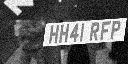 expected output
HH41RFP 1.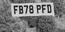 expected output
FB78PFD 1.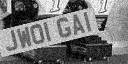 expected output
JW01GAI 0. (Plate partially truncated.)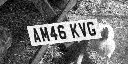 expected output
AM46KVG 0. (Plate too small.)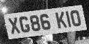 expected output
XG86KIO 0. (Plate too big.) expected output
XH07NYO 0. (Plate not present at all.)
The process for generating the images is illustrated below:
The text and plate colour are chosen randomly, but the text must be a certain amount darker than the plate. This is to simulate real-world lighting variation. Noise is added at the end not only to account for actual sensor noise, but also to avoid the network depending too much on sharply defined edges as would be seen with an out-of-focus input image.
Having a background is important as it means the network must learn to identify the bounds of the number plate without “cheating”: Were a black background used for example, the network may learn to identify plate location based on non-blackness, which would clearly not work with real pictures of cars.
The backgrounds are sourced from the SUN database, which contains over 100,000 images. It’s important the number of images is large to avoid the network “memorizing” background images.
The transformation applied to the plate (and its mask) is an affine transformation based on a random roll, pitch, yaw, translation, and scale. The range allowed for each parameter was selected according to the ranges that number plates are likely to be seen. For example, yaw is allowed to vary a lot more than roll (you’re more likely to see a car turning a corner, than on its side).
The code to generate the images is relatively short (~300 lines). It can be read in gen.py.
The network
Here’s the network architecture used:See the wikipedia page for a summary of CNN building blocks. The above network is in fact based on this paper by Stark et al, as it gives more specifics about the architecture used than the Google paper.
The output layer has one node (shown on the left) which is used as the presence indicator. The rest encode the probability of a particular number plate: Each column as shown in the diagram corresponds with one of the digits in the number plate, and each node gives the probability of the corresponding character being present. For example, the node in column 2 row 3 gives the probability that the second digit is a
C.As is standard with deep neural nets all but the output layers use ReLU activation. The presence node has sigmoid activation as is typically used for binary outputs. The other output nodes use softmax across characters (ie. so that the probability in each column sums to one) which is the standard approach for modelling discrete probability distributions.
The code defining the network is in model.py.
The loss function is defined in terms of the cross-entropy between the label and the network output. For numerical stability the activation functions of the final layer are rolled into the cross-entropy calculation using
softmax_cross_entropy_with_logits and
sigmoid_cross_entropy_with_logits. For a
detailed and intuitive introduction to cross-entropy see this section
in Michael A. Nielsen’s free online book.Training (train.py) takes about 6 hours using a nVidia GTX 970, with training data being generated on-the-fly by a background process on the CPU.
Output Processing
To actually detect and recognize number plates in an input image a network much like the above is applied to 128x64 windows at various positions and scales, as described in the windowing section.The network differs from the one used in training in that the last two layers are convolutional rather than fully connected, and the input image can be any size rather than 128x64. The idea is that the whole image at a particular scale can be fed into this network which yields an image with a presence / character probability values at each “pixel”. The idea here is that adjacent windows will share many convolutional features, so rolling them into the same network avoids calculating the same features multiple times.
Visualizing the “presence” portion of the output yields something like the following:
Image credit
The boxes here are regions where the network detects a greater than 99% probability that a number plate is present. The reason for the high threshold is to account for a bias introduced in training: About half of the training images contained a number plate, whereas in real world images of cars number plates are much rarer. As such if a 50% threshold is used the detector is prone to false positives.
To cope with the obvious duplicates we apply a form of non-maximum suppression to the output:
Image credit
The technique used here first groups the rectangles into overlapping rectangles, and for each group outputs:
- The intersection of all the bounding boxes.
- The license number corresponding with the box in the group that had the highest probability of being present.
Image credit
Whoops, the R has been misread as a P. Here’s the window from the above image which gives the maximum presence response:
Image credit
On first glance it appears that this should be an easy case for the detector, however it turns out to be an instance of overfitting. Here’s the R from the number plate font used to generate the training images:
Note how the leg of the R is at a different angle to the leg of the R in the input image. The network has only ever seen R’s as shown above, so gets confused when it sees R’s in a different font. To test this hypothesis I modified the image in GIMP to more closely resemble the training font:
And sure enough, the detector now gets the correct result:
The code for the detector is in detect.py.
Conclusion
I’ve shown that with a relatively short amount of code (~800 lines), its possible to build an ANPR system without importing any domain-specific libraries, and with very little domain-specific knowledge. Furthermore I’ve side-stepped the problem of needing thousands of training images (as is usually the case with deep neural networks) by synthesizing images on the fly.On the other hand, my system has a number of drawbacks:
-
It only works with number plates in a specific format. More specifically,
the network architecture assumes exactly 7 chars are visible in the output.
-
It only works on specific number plate fonts.
-
It’s slow. The system takes several seconds to run on moderately sized
image.
I showed an instance of 2) above, with the misdetection of an R due to a slightly varied font. The effects would be further exacerbated if I were trying to detect US number plates rather than UK number plates which have much more varied fonts. One possible solution would be to make my training data more varied by drawing from a selection of fonts, although it’s not clear how many fonts I would need for this approach to be successful.
The slowness (3)) is a killer for many applications: A modestly sized input image takes a few seconds to process on a reasonably powerful GPU. I don’t think its possible to get away from this without introducing a (cascade of) detection stages, for example a Haar cascade, a HOG detector, or a simpler neural net.
It would be an interesting exercise to see how other ML techniques compare, in particular pose regression (with the pose being an affine transformation corresponding with 3 corners of the plate) looks promising. A much more basic classification stage could then be tacked on the end. This solution should be similarly terse if an ML library such as scikit-learn is used.
In conclusion, I’ve shown that a single CNN (with some filtering) can be used as a passable number plate detector / recognizer, however it does not yet compete with the traditional hand-crafted (but more verbose) pipelines in terms of performance.
Image Credits
Original “Proton Saga EV” image by Somaditya Bandyopadhyay licensed under the Creative Commons Attribution-Share Alike 2.0 Generic license.
Original “Google Street View Car” image by Reedy licensed under the Creative Commons Attribution-Share Alike 3.0 Unported license.
Monday, May 2, 2016
Sketch Simplification
http://hi.cs.waseda.ac.jp/~esimo/en/research/sketch/#

 Our model is based on a fully convolutional neural network. We input the model a
rough sketch image and obtain as an output a clean simplified sketch. This is done by
processing the image with convolutional layers, which can be seen as banks of filters
that are run on the input. While the input is a grayscale image, our model internally
uses a much larger representation. We build the model upon three different types of
convolutions: down-convolution, halves the resolution by using a stride of two;
flat-convolutional, processes the image without changing the resolution; and
up-convolution, doubles the resolution by using a stride of one half. This allows our
model to initially compress the image into a smaller representation, process the small
image, and finally expand it into the simplified clean output image that can easily be
vectorized.
Our model is based on a fully convolutional neural network. We input the model a
rough sketch image and obtain as an output a clean simplified sketch. This is done by
processing the image with convolutional layers, which can be seen as banks of filters
that are run on the input. While the input is a grayscale image, our model internally
uses a much larger representation. We build the model upon three different types of
convolutions: down-convolution, halves the resolution by using a stride of two;
flat-convolutional, processes the image without changing the resolution; and
up-convolution, doubles the resolution by using a stride of one half. This allows our
model to initially compress the image into a smaller representation, process the small
image, and finally expand it into the simplified clean output image that can easily be
vectorized.
 We evaluate extensively on complicated real scanned sketches and show that our
approach is able to significantly outperform the state of the art. We corroborate
results with a user test in which we see that our model significantly outperforms
vectorization approaches. Images (a), (b), and (d) are part of our test set, while
images (c) and (e) were taken from Flickr. Image (c) courtesy of Anna Anjos and image
(e) courtesy of Yama Q under creative commons licensing.
We evaluate extensively on complicated real scanned sketches and show that our
approach is able to significantly outperform the state of the art. We corroborate
results with a user test in which we see that our model significantly outperforms
vectorization approaches. Images (a), (b), and (d) are part of our test set, while
images (c) and (e) were taken from Flickr. Image (c) courtesy of Anna Anjos and image
(e) courtesy of Yama Q under creative commons licensing.
 We perform a user study and compare against vectorization tools that work directly
on raster images. In particular we consider the open-source Potrace and the commercial Adobe Live Trace.
Users prefer our approach over 97% of the time with respect to either of the two
tools.
We perform a user study and compare against vectorization tools that work directly
on raster images. In particular we consider the open-source Potrace and the commercial Adobe Live Trace.
Users prefer our approach over 97% of the time with respect to either of the two
tools.
For more details and results, please consult the full paper.

Sketch Simplification
We present a novel technique to simplify sketch drawings based on learning a series of
convolution operators. In contrast to existing approaches that require vector images as
input, we allow the more general and challenging input of rough raster sketches such as
those obtained from scanning pencil sketches. We convert the rough sketch into a
simplified version which is then amendable for vectorization. This is all done in a fully
automatic way without user intervention. Our model consists of a fully convolutional
neural network which, unlike most existing convolutional neural networks, is able to
process images of any dimensions and aspect ratio as input, and outputs a simplified
sketch which has the same dimensions as the input image. In order to teach our model to
simplify, we present a new dataset of pairs of rough and simplified sketch drawings. By
leveraging convolution operators in combination with efficient use of our proposed
dataset, we are able to train our sketch simplification model. Our approach naturally
overcomes the limitations of existing methods, e.g., vector images as input and long
computation time; and we show that meaningful simplifications can be obtained for many
different test cases. Finally, we validate our results with a user study in which we
greatly outperform similar approaches and establish the state of the art in sketch
simplification of raster images.
Model
Results
Comparison
For more details and results, please consult the full paper.
Publications
2016
- Learning to Simplify: Fully Convolutional Networks for Rough Sketch Cleanup
- ACM Transactions on Graphics (SIGGRAPH), 2016
Subscribe to:
Posts (Atom)