Thursday, December 21, 2017

Challenge : Pover-T Tests: Predicting Poverty

https://www.drivendata.org/competitions/50/worldbank-poverty-prediction/page/97/

Predicting Poverty - World Bank

The World Bank is aiming to end extreme poverty by 2030. Crucial to this goal are techniques for determining which poverty reduction strategies work and which ones do not. But measuring poverty reduction requires measuring poverty in the first place, and it turns out that measuring poverty is pretty hard. The World Bank helps developing countries measure poverty by conducting in-depth household surveys with a subset of the country's population. To measure poverty, most of these surveys collect detailed data on household consumption – everything from food and transportation habits to healthcare access and sporting events – in order to get a clearer picture of a household's poverty status.
Can you harness the power of these data to identify the strongest predictors of poverty? Right now measuring poverty is hard, time consuming, and expensive. By building better models, we can run surveys with fewer, more targeted questions that rapidly and cheaply measure the effectiveness of new policies and interventions. The more accurate our models, the more accurately we can target interventions and iterate on policies, maixmizing the impact and cost-effectiveness of these strategies.

Machine Tagging Challenge

https://www.innocentive.com/ar/challenge/9934063

The Seeker desires an algorithm to map customer-supplied tag names for data sources onto Seeker-defined Standard Tags. The algorithm must perform the mapping operation without human intervention and must be able to adapt to new data as it becomes available.
This is a Reduction-to-Practice Challenge that requires written documentation, output from the algorithm, and submission of working software and source code implementing the solution.


Wednesday, December 20, 2017

WWW 2018 Challenge: Learning to Recognize Musical Genre

https://www.crowdai.org/challenges/www-2018-challenge-learning-to-recognize-musical-genre

Overview

Like never before, the web has become a place for sharing creative work - such as music - among a global community of artists and art lovers. While music and music collections predate the web, the web enabled much larger scale collections. Whereas people used to own a handful of vinyls or CDs, they nowadays have instant access to the whole of published musical content via online platforms. Such dramatic increase in the size of music collections created two challenges: (i) the need to automatically organize a collection (as users and publishers cannot manage them manually anymore), and (ii) the need to automatically recommend new songs to a user knowing his listening habits. An underlying task in both those challenges is to be able to group songs in semantic categories.
Music genres are categories that have arisen through a complex interplay of cultures, artists, and market forces to characterize similarities between compositions and organize music collections. Yet, the boundaries between genres still remain fuzzy, making the problem of music genre recognition (MGR) a nontrivial task (Scaringella 2006). While its utility has been debated, mostly because of its ambiguity and cultural definition, it is widely used and understood by end-users who find it useful to discuss musical categories (McKay 2006). As such, it is one of the most researched areas in the Music Information Retrieval (MIR) field (Sturm 2012).
The task of this challenge, one of the four official challenges of the Web Conference (WWW2018) challenges track, is to recognize the musical genre of a piece of music of which only a recording is available. Genres are broad, e.g. pop or rock, and each song only has one target genre. The data for this challenge comes from the recently published FMA dataset (Defferrard 2017), which is a dump of the Free Music Archive (FMA), an interactive library of high-quality and curated audio which is freely and openly available to the public.

Friday, December 15, 2017

Visual Domain Decathlon Challenge

http://www.robots.ox.ac.uk/~vgg/decathlon/

Part of PASCAL in Detail Workshop Challenge, CVPR 2017, July 26th, Honolulu, Hawaii, USA
This taster challenge tests the ability of visual recognition algorithms to cope with (or take advantage of) many different visual domains.

Thursday, November 23, 2017

Understanding SSD MultiBox — Real-Time Object Detection In Deep Learning

https://towardsdatascience.com/understanding-ssd-multibox-real-time-object-detection-in-deep-learning-495ef744fab

This post is meant to constitute an intuitive explanation of the SSD MultiBox object detection technique. I have tried to minimise the maths and instead slowly guide you through the tenets of this architecture, which includes explaining what the MultiBox algorithm does. After reading this post, I hope you will have a better grasp of SSD and will try it out for yourselves!

Since AlexNet took the research world by storm at the 2012 ImageNet Large-Scale Visual Recognition Challenge (ILSVRC), deep learning has become the go-to method for image recognition tasks, far surpassing more traditional computer vision methods used in the literature. In the field of computer vision, convolution neural networks excel at image classification, which consists of categorising images, given a set of classes (e.g. cat, dog), and having the network determine the strongest class present in the image.
Images of cats and dogs (from kaggle)
Nowadays, deep learning networks are better at image classification than humans, which shows just how powerful this technique is. However, we as humans do far more than just classify images when observing and interacting with the world. We also localize and classify each element within our field of view. These are much more complex tasks which machines are still struggling to perform as well as humans. In fact, I would argue that object detection when performed well, brings machines closer to real scene understanding.
Does the image show cat, a dog, or do we have both? (from kaggle)

The Region-Convolutional Neural Network (R-CNN)

A few years ago, by exploiting some of the leaps made possible in computer vision via CNNs, researchers developed R-CNNs to deal with the tasks of object detection, localization and classification. Broadly speaking, a R-CNN is a special type of CNN that is able to locate and detect objects in images: the output is generally a set of bounding boxes that closely match each of the detected objects, as well as a class output for each detected object. The image below shows what a typical R-CNN outputs:
Example output of R-CNN
There is an exhaustive list of papers in this field and for anyone eager to explore further I recommend starting with the following “trilogy” of papers around the topic:
As you might have guessed, each next paper proposes improvements to the seminal work done in R-CNN to develop a faster network, with the goal of achieving real-time object detection. The achievements displayed through this set of work is truly amazing, yet none of these architectures manage to create a real-time object detector. Without going too much into details, the following problems with the above networks were identified:
  • Training the data is unwieldy and too long
  • Training happens in multiple phases (e.g. training region proposal vs classifier)
  • Network is too slow at inference time (i.e. when dealing with non-training data)
Fortunately, in the last few years, new architectures were created to address the bottlenecks of R-CNN and its successors, enabling real-time object detection. The most famous ones are YOLO (You Only Look Once) and SSD MultiBox (Single Shot Detector). In this post, we will discuss SSD as there seem to be less coverage about this architecture than YOLO. Besides, you should also find it easier to grasp YOLO once you understand SSD.

Single Shot MultiBox Detector

The paper about SSD: Single Shot MultiBox Detector (by C. Szegedy et al.) was released at the end of November 2016 and reached new records in terms of performance and precision for object detection tasks, scoring over 74% mAP (mean Average Precision) at 59 frames per second on standard datasets such as PascalVOC and COCO. To better understand SSD, let’s start by explaining where the name of this architecture comes from:
  • Single Shot: this means that the tasks of object localization and classification are done in a single forward pass of the network
  • MultiBox: this is the name of a technique for bounding box regression developed by Szegedy et al. (we will briefly cover it shortly)
  • Detector: The network is an object detector that also classifies those detected objects

Architecture

Architecture of Single Shot MultiBox detector (input is 300x300x3)
As you can see from the diagram above, SSD’s architecture builds on the venerable VGG-16 architecture, but discards the fully connected layers. The reason VGG-16 was used as the base network is because of its strong performance in high quality image classification tasks and its popularity for problems where transfer learning helps in improving results. Instead of the original VGG fully connected layers, a set of auxiliary convolutional layers (from conv6 onwards) were added, thus enabling to extract features at multiple scales and progressively decrease the size of the input to each subsequent layer.
VGG architecture (input is 224x224x3)

MultiBox

The bounding box regression technique of SSD is inspired by Szegedy’s work on MultiBox, a method for fast class-agnostic bounding box coordinate proposals. Interestingly, in the work done on MultiBox an Inception-style convolutional network is used. The 1x1 convolutions that you see below help in dimensionality reduction since the number of dimensions will go down (but “width” and “height” will remain the same).
Architecture of multi-scale convolutional prediction of the location and confidences of multibox
MultiBox’s loss function also combined two critical components that made their way into SSD:
  • Confidence Loss: this measures how confident the network is of the objectness of the computed bounding box. Categorical cross-entropy is used to compute this loss.
  • Location Loss: this measures how far away the network’s predicted bounding boxes are from the ground truth ones from the training set. L2-Norm is used here.
Without delving too deep into the math (read the paper if you are curious and want a more rigorous notation), the expression for the loss, which measures how far off our prediction “landed”, is thus:
multibox_loss = confidence_loss + alpha * location_loss
The alpha term helps us in balancing the contribution of the location loss. As usual in deep learning, the goal is to find the parameter values that most optimally reduce the loss function, thereby bringing our predictions closer to the ground truth.

MultiBox Priors And IoU

The logic revolving around the bounding box generation is actually more complex than what I earlier stated. But fear not: it is still within reach.
In MultiBox, the researchers created what we call priors (or anchors in Faster-R-CNN terminology), which are pre-computed, fixed size bounding boxes that closely match the distribution of the original ground truth boxes. In fact those priors are selected in such a way that their Intersection over Union ratio (aka IoU, and sometimes referred to as Jaccard index) is greater than 0.5. As you can infer from the image below, an IoU of 0.5 is still not good enough but it does however provide a strong starting point for the bounding box regression algorithm — it is a much better strategy than starting the predictions with random coordinates! Therefore MultiBox starts with the priors as predictions and attempt to regress closer to the ground truth bounding boxes.
Diagram explaining IoU (from Wikipedia)
The resulting architecture (check MultiBox architecture diagram above again for reference) contains 11 priors per feature map cell (8x8, 6x6, 4x4, 3x3, 2x2) and only one on the 1x1 feature map, resulting in a total of 1420 priors per image, thus enabling robust coverage of input images at multiple scales, to detect objects of various sizes.
At the end, MultiBox only retains the top K predictions that have minimised both location (LOC) and confidence (CONF) losses.

SSD Improvements

Back onto SSD, a number of tweaks were added to make this network even more capable of localizing and classifying objects.
Fixed Priors: unlike MultiBox, every feature map cell is associated with a set of default bounding boxes of different dimensions and aspect ratios. These priors are manually (but carefully) chosen, whereas in MultiBox, they were chosen because their IoU with respect to the ground truth was over 0.5. This in theory should allow SSD to generalise for any type of input, without requiring a pre-training phase for prior generation. For instance, assuming we have configured b default bounding boxes per feature map cell, and c classes to classify, on a given feature map of size f = m x n, SSD would compute f(b + c) values for this feature map.
SSD default boxes at 8x8 and 4x4 feature maps
Location Loss: SSD uses smooth L1-Norm to calculate the location loss. While not as precise as L2-Norm, it is still highly effective and gives SSD more room for manoeuvre as it does not try to be “pixel perfect” in its bounding box prediction (i.e. a difference of a few pixels would hardly be noticeable for many of us).
Classification: MultiBox does not perform object classification, whereas SSD does. Therefore, for each predicted bounding box, a set of c class predictions are computed, for every possible class in the dataset.

Training & Running SSD

Datasets

You will need training and test datasets with ground truth bounding boxes and assigned class labels (only one per bounding box). The Pascal VOC and COCO datasets are a good starting point.
Images from Pascal VOC dataset

Default Bounding Boxes

It is recommended to configure a varied set of default bounding boxes, of different scales and aspect ratios to ensure most objects could be captured. The SSD paper has around 6 bounding boxes per feature map cell.

Feature Maps

Features maps (i.e. the results of the convolutional blocks) are a representation of the dominant features of the image at different scales, therefore running MultiBox on multiple feature maps increases the likelihood of any object (large and small) to be eventually detected, localized and appropriately classified. The image below shows how the network “sees” a given image across its feature maps:
VGG Feature Map Visualisation (from Brown Uni)

Hard Negative Mining

During training, as most of the bounding boxes will have low IoU and therefore be interpreted as negative training examples, we may end up with a disproportionate amount of negative examples in our training set. Therefore, instead of using all negative predictions, it is advised to keep a ratio of negative to positive examples of around 3:1. The reason why you need to keep negative samples is because the network also needs to learn and be explicitly told what constitutes an incorrect detection.
Example of hard negative mining (from Jamie Kang blog)

Data Augmentation

The authors of SSD stated that data augmentation, like in many other deep learning applications, has been crucial to teach the network to become more robust to various object sizes in the input. To this end, they generated additional training examples with patches of the original image at different IoU ratios (e.g. 0.1, 0.3, 0.5, etc.) and random patches as well. Moreover, each image is also randomly horizontally flipped with a probability of 0.5, thereby making sure potential objects appear on left and right with similar likelihood.
Example of horizontally flipped image (from Behavioural Cloning blog post)

Non-Maximum Suppression (NMS)

Given the large number of boxes generated during a forward pass of SSD at inference time , it is essential to prune most of the bounding box by applying a technique known as non-maximum suppression: boxes with a confidence loss threshold less than ct (e.g. 0.01) and IoU less than lt (e.g. 0.45) are discarded, and only the top N predictions are kept. This ensures only the most likely predictions are retained by the network, while the more noisier ones are removed.
NMS example (from DeepHub tweet)

Additional Notes On SSD

The SSD paper makes the following additional observations:
  • more default boxes results in more accurate detection, although there is an impact on speed
  • having MultiBox on multiple layers results in better detection as well, due to the detector running on features at multiple resolutions
  • 80% of the time is spent on the base VGG-16 network: this means that with a faster and equally accurate network SSD’s performance could be even better
  • SSD confuses objects with similar categories (e.g. animals). This is probably because locations are shared for multiple classes
  • SSD-500 (the highest resolution variant using 512x512 input images) achieves best mAP on Pascal VOC2007 at 76.8%, but at the expense of speed, where its frame rate drops to 22 fps. SSD-300 is thus a much better trade-off with 74.3 mAP at 59 fps.
  • SSD produces worse performance on smaller objects, as they may not appear across all feature maps. Increasing the input image resolution alleviates this problem but does not completely address it

Playing With SSD

There are a few implementations of SSD available online, including the original Caffe code from the authors of the paper. In my case, I opted for Paul Balança’s TensorFlow implementation, available on github. It is worth reading the code as well the paper to better understand how everything fits together.
I also recently decided to reimplement a project on Vehicle Detection that was using traditional computer vision techniques, by employing SSD this time. A small gif of my output using SSD shows it works very well:
GIF of vehicle detection Using SSD

Beyond SSD

More recent work in this field has been produced, and I would recommend following up on the two papers below for anyone interested in pushing their knowledge further in this domain:
Voilà! We are done with our tour of Single Shot MultiBox Detector. I tried to explain the concepts behind this technique in simple terms, as best as I understood them, with many pictures to further illustrate those concepts and facilitate your understanding. I do really recommend reading the paper (probably a few times if you are slow like me 🙃), including forming good intuition behind some of the maths in this technique to cement your comprehension. You can always check this post if some of its sections help you make sense of the paper. Godspeed!

Monday, November 20, 2017

VLBI Reconstruction Dataset

http://vlbiimaging.csail.mit.edu/

Welcome to the VLBI Reconstruction Dataset!

The goal of this website is to provide a testbed for developing new VLBI reconstruction algorithms. By supplying a large set of easy to understand training and testing data, we hope to make the problem more accessible to those less familiar with the VLBI field. Specifically, this website contains a:

What is VLBI Imaging?

Imaging distant celestial sources with high resolving power requires telescopes with prohibitively large diameters due to the inverse relationship between angular resolution and telescope diameter. However, by simultaneously collecting data from an array of telescopes located around the Earth, it is possible to emulate samples from a single telescope with a diameter equal to the maximum distance between telescopes in the array. Using multiple telescopes in this manner is referred to as very long baseline interferometry (VLBI).
Reconstructing an image using VLBI measurements is an ill-posed problem, and as such each there are an infinite number of possible images that explain the data. The challenge is to find an explanation that respects these prior assumptions while still satisfying the observed data. The goal of this website to aid in the process of developing these algorithms as well as evaluate their performance.

The ongoing international effort to create an Event Horizon Telescope capable of imaging the enviroment around a black hole’s event horizon calls for the use of VLBI reconstruction algorithms. The angular resolution necessary for these measurements requires overcoming many challenges, all of which make image reconstruction more difficult. For instance, at the mm/sub-mm wavelengths being observed, rapidly varying inhomogeneities in the atmosphere introduce additional measurement errors. Robust algorithms that are able to reconstruct images in this fine angular resolution regime are essential for scientific progress.

Tuesday, November 7, 2017

Theories of Deep Learning (STATS 385)

https://stats385.github.io/

The spectacular recent successes of deep learning are purely empirical. Nevertheless intellectuals always try to explain important developments theoretically. In this literature course we will review recent work of Bruna and Mallat, Mhaskar and Poggio, Papyan and Elad, Bolcskei and co-authors, Baraniuk and co-authors, and others, seeking to build theoretical frameworks deriving deep networks as consequences. After initial background lectures, we will have some of the authors presenting lectures on specific papers. This course meets once weekly.

Cheat Sheets for AI Neural Networks Machine Learning Deep Learning Big Data

https://becominghuman.ai/cheat-sheets-for-ai-neural-networks-machine-learning-deep-learning-big-data-678c51b4b463

The Most Complete List of Best AI Cheat Sheets

Over the past few months, I have been collecting AI cheat sheets. From time to time I share them with friends and colleagues and recently I have been getting asked a lot, so I decided to organize and share the entire collection. To make things more interesting and give context, I added descriptions and/or excerpts for each major topic.
This is the most complete list and the Big-O is at the very end, enjoy…

Thursday, October 5, 2017

A Comprehensive guide to Fine-tuning Deep Learning Models in Keras (Part II)

https://flyyufelix.github.io/2016/10/08/fine-tuning-in-keras-part2.html

This is Part II of a 2 part series that cover fine-tuning deep learning models in Keras. Part I states the motivation and rationale behind fine-tuning and gives a brief introduction on the common practices and techniques. This post will give a detailed step-by-step guide on how to go about implementing fine-tuning on popular models VGG, Inception, and ResNet in Keras.

Why do we pick Keras?

Keras is a simple to use neural network library built on top of Theano or TensorFlow that allows developers to prototype ideas very quickly. Unless you are doing some cutting-edge research that involves customizing a completely novel neural architecture with different activation mechanism, Keras provides all the building blocks you need to build reasonably sophisticated neural networks.
It also comes with a great documentation and tons of online resources.

Note on Hardware

I would strongly suggest getting a GPU to do the heavy computation involved in Covnet training. The speed difference is very substantial. We are talking about a matter of hours with a GPU versus a matter of days with a CPU.
I would recommend GTX 980Ti or a slightly expensive GTX 1080 which cost around $600 bucks.

Fine-tuning in Keras

I have implemented starter scripts for fine-tuning convnets in Keras. The scripts are hosted in this github page. Implementations of VGG16, VGG19, GoogLeNet, Inception-V3, and ResNet50 are included. With that, you can customize the scripts for your own fine-tuning task.
Below is a detailed walkthrough of how to fine-tune VGG16 and Inception-V3 models using the scripts.
Fine-tune VGG16. VGG16 is a 16-layer Covnet used by the Visual Geometry Group (VGG) at Oxford University in the 2014 ILSVRC (ImageNet) competition. The model achieves a 7.5% top 5 error rate on the validation set, which is a result that earned them a second place finish in the competition.
Schematic Diagram of VGG16 Model:
VGG16 Model
The script for fine-tuning VGG16 can be found in vgg16.py. The first part of the vgg_std16_model function is the model schema for VGG16. After defining the fully connected layer, we load the ImageNet pre-trained weight to the model by the following line:
model.load_weights('cache/vgg16_weights.h5')
For fine-tuning purpose, we truncate the original softmax layer and replace it with our own by the following snippet:
model.layers.pop()
model.outputs = [model.layers[-1].output]
model.layers[-1].outbound_nodes = []
model.add(Dense(num_class, activation='softmax'))
Where the num_class variable in the last line represents the number of class labels for our classification task.
Sometimes, we want to freeze the weight for the first few layers so that they remain intact throughout the fine-tuning process. Say we want to freeze the weights for the first 10 layers. This can be done by the following lines:
for layer in model.layers[:10]:
    layer.trainable = False
We then fine-tune the model by minimizing the cross entropy loss function using stochastic gradient descent (sgd) algorithm. Notice that we use an initial learning rate of 0.001, which is smaller than the learning rate for training scratch model (usually 0.01).
sgd = SGD(lr=1e-3, decay=1e-6, momentum=0.9, nesterov=True)
model.compile(optimizer=sgd, loss='categorical_crossentropy', metrics=['accuracy'])
model = vgg_std16_model(img_rows, img_cols, channel, num_class)
Where img_rows, img_cols, and channel define the dimension of the input. For colored image with resolution 224x224, img_rows = img_cols = 224, channel = 3.
Next, we load our dataset, split it into training and testing sets, and start fine-tuning the model:
X_train, X_valid, Y_train, Y_valid = load_data()

model.fit(train_data, test_data,
          batch_size=batch_size,
          nb_epoch=nb_epoch,
          shuffle=True,
          verbose=1,
          validation_data=(X_valid, Y_valid),
          )
The fine-tuning process will take a while, depending on your hardware. After it is done, we use the model the make prediction on the validation set and return the score for the cross entropy loss:
predictions_valid = model.predict(X_valid, batch_size=batch_size, verbose=1)
score = log_loss(Y_valid, predictions_valid)
Fine-tune Inception-V3. Inception-V3 achieved the second place in the 2015 ImageNet competition with a 5.6% top 5 error rate on the validation set. The model is characterized by the usage of the Inception Module, which is a concatenation of features maps generated by kernels of varying dimensions.
Schematic Diagram of the 27-layer Inception-V1 Model (Idea similar to that of V3):
Inception-V1 Model
The code for fine-tuning Inception-V3 can be found in inception_v3.py. The process is mostly similar to that of VGG16, with one subtle difference. Inception-V3 does not use Keras’ Sequential Model due to branch merging (for the inception module), hence we cannot simply use model.pop() to truncate the top layer.
Instead, after we create the model and load it up with the ImageNet weight, we perform the equivalent of top layer truncation by defining another fully connected sofmax (x_newfc) on top of the last inception module (x). This is done using the following snippet:
# Last Inception Module 
x = merge([branch1x1, branch3x3, branch3x3dbl, branch_pool],
                  mode='concat', concat_axis=channel_axis,
                  name='mixed' + str(9 + i))

# Fully Connected Softmax Layer
x_fc = AveragePooling2D((8, 8), strides=(8, 8), name='avg_pool')(x)
x_fc = Flatten(name='flatten')(x_fc)
x_fc = Dense(1000, activation='softmax', name='predictions')(x_fc)

# Create model
model = Model(img_input, x_fc)

# Load ImageNet pre-trained data
model.load_weights('cache/inception_v3_weights_th_dim_ordering_th_kernels.h5')

# Truncate and replace softmax layer for transfer learning
# Cannot use model.layers.pop() since model is not of Sequential() type
# The method below works since pre-trained weights are stored in layers but not in the model
x_newfc = AveragePooling2D((8, 8), strides=(8, 8), name='avg_pool')(x)
x_newfc = Flatten(name='flatten')(x_newfc)

# Create another model with our customized softmax
model = Model(img_input, x_newfc)

# Learning rate is changed to 0.001
sgd = SGD(lr=1e-3, decay=1e-6, momentum=0.9, nesterov=True)
model.compile(optimizer=sgd, loss='categorical_crossentropy', metrics=['accuracy'])
model = inception_v3_model(img_rows, img_cols, channel, num_class)
That’s it for Inception-V3. Starting script for other models such as VGG19, GoogleLeNet, and ResNet can be found here.

Fine-tuned Networks in Action

If you are a Deep Learning or Computer Vision practitioner, most likely you have already tried fine-tuning pre-trained network for your own classification problem before.
To me, I came across this interesting Kaggle Competition which requires candidates to identify distracted drivers through analyzing in-car camera images. This is a good opportunity for me to try out fine-tuning in Keras.
Following the fine-tuning methods listed above, together with data preprocessing/augmentation and model ensembling our team managed to achieved top 4% in the competition. Detailed account of our method and lessons learned are captured in this post.
If you have any questions or thoughts feel free to leave a comment below.
You can also follow me on Twitter at @flyyufelix.

Monday, September 25, 2017

An Intuitive Explanation of Convolutional Neural Networks

https://ujjwalkarn.me/2016/08/11/intuitive-explanation-convnets/

What are Convolutional Neural Networks and why are they important?

Convolutional Neural Networks (ConvNets or CNNs) are a category of Neural Networks that have proven very effective in areas such as image recognition and classification. ConvNets have been successful in identifying faces, objects and traffic signs apart from powering vision in robots and self driving cars.
Screen Shot 2017-05-28 at 11.41.55 PM.png
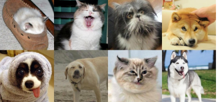
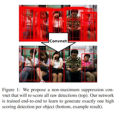
Figure 1: Source [1]
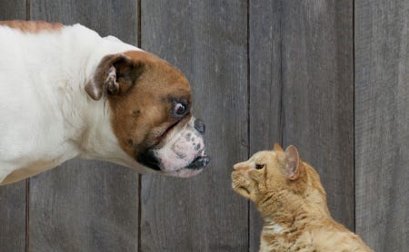
In Figure 1 above, a ConvNet is able to recognize scenes and the system is able to suggest relevant captions (“a soccer player is kicking a soccer ball”) while Figure 2 
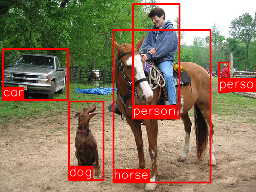
shows an example of ConvNets being used for recognizing everyday objects, humans and animals. Lately, ConvNets have been effective in several Natural Language Processing tasks (such as sentence classification) as well.
Screen Shot 2016-08-07 at 4.17.11 PM.png
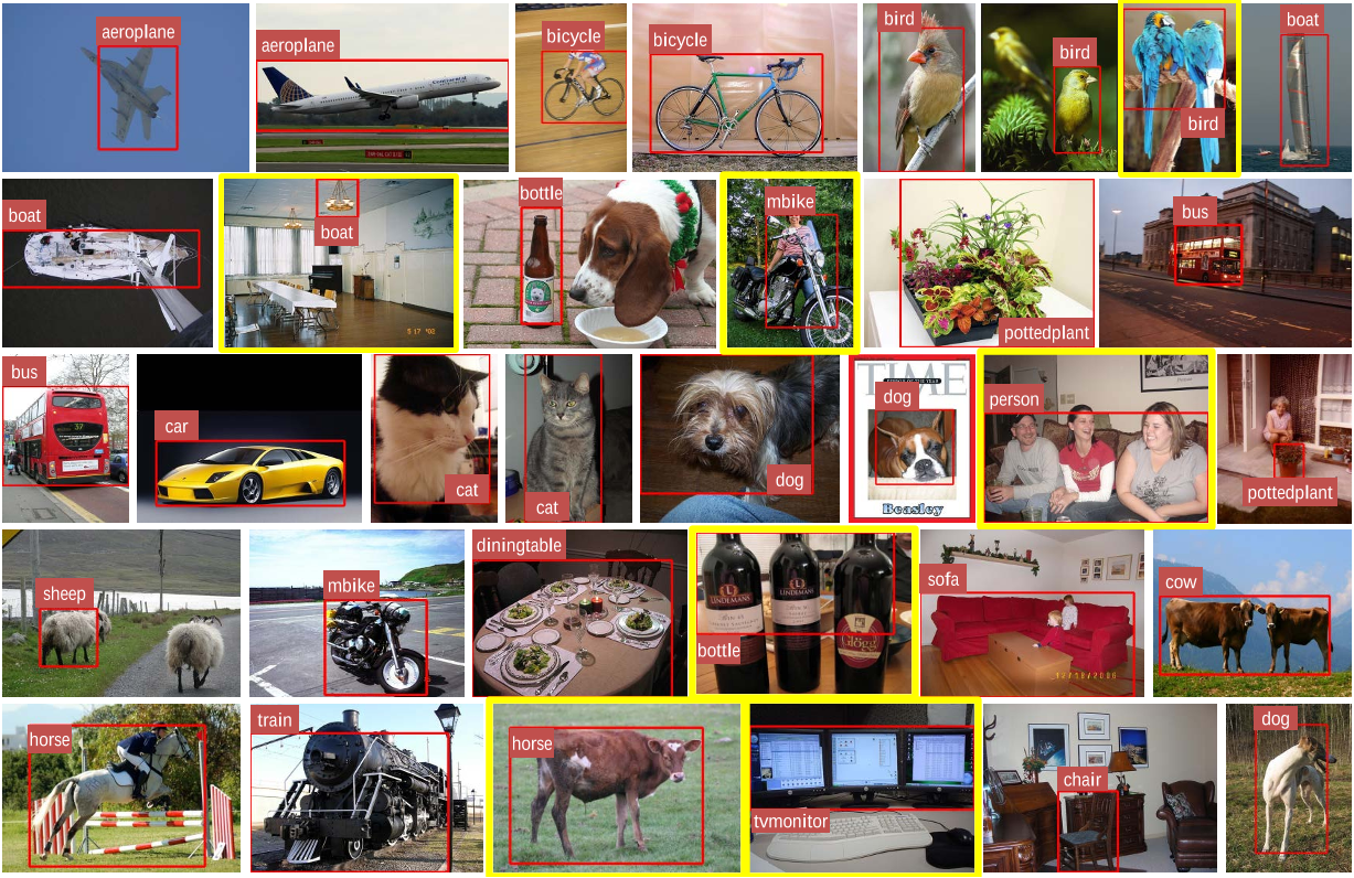
Figure 2: Source [2]
ConvNets, therefore, are an important tool for most machine learning practitioners today. However, understanding ConvNets and learning to use them for the first time can sometimes be an intimidating experience. The primary purpose of this blog post is to develop an understanding of how Convolutional Neural Networks work on images.
If you are new to neural networks in general, I would recommend reading this short tutorial on Multi Layer Perceptrons to get an idea about how they work, before proceeding. Multi Layer Perceptrons are referred to as “Fully Connected Layers” in this post.

The LeNet Architecture (1990s)

LeNet was one of the very first convolutional neural networks which helped propel the field of Deep Learning. This pioneering work by Yann LeCun was named LeNet5 after many previous successful iterations since the year 1988 [3]. At that time the LeNet architecture was used mainly for character recognition tasks such as reading zip codes, digits, etc.
Below, we will develop an intuition of how the LeNet architecture learns to recognize images. There have been several new architectures proposed in the recent years which are improvements over the LeNet, but they all use the main concepts from the LeNet and are relatively easier to understand if you have a clear understanding of the former.
Screen Shot 2016-08-07 at 4.59.29 PM.png
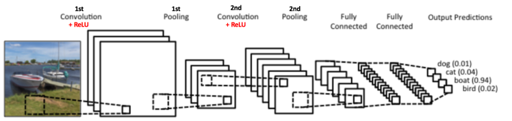
Figure 3: A simple ConvNet. Source [5]
The Convolutional Neural Network in Figure 3 is similar in architecture to the original LeNet and classifies an input image into four categories: dog, cat, boat or bird (the original LeNet was used mainly for character recognition tasks). As evident from the figure above, on receiving a boat image as input, the network correctly assigns the highest probability for boat (0.94) among all four categories. The sum of all probabilities in the output layer should be one (explained later in this post).
There are four main operations in the ConvNet shown in Figure 3 above:
  1. Convolution
  2. Non Linearity (ReLU)
  3. Pooling or Sub Sampling
  4. Classification (Fully Connected Layer)
These operations are the basic building blocks of every Convolutional Neural Network, so understanding how these work is an important step to developing a sound understanding of ConvNets. We will try to understand the intuition behind each of these operations below.

An Image is a matrix of pixel values

Essentially, every image can be represented as a matrix of pixel values.
8-gif.gif
Figure 4: Every image is a matrix of pixel values. Source [6]
Channel is a conventional term used to refer to a certain component of an image. An image from a standard digital camera will have three channels – red, green and blue – you can imagine those as three 2d-matrices stacked over each other (one for each color), each having pixel values in the range 0 to 255.
grayscale image, on the other hand, has just one channel. For the purpose of this post, we will only consider grayscale images, so we will have a single 2d matrix representing an image. The value of each pixel in the matrix will range from 0 to 255 – zero indicating black and 255 indicating white.

The Convolution Step

ConvNets derive their name from the “convolution” operator. The primary purpose of Convolution in case of a ConvNet is to extract features from the input image. Convolution preserves the spatial relationship between pixels by learning image features using small squares of input data. We will not go into the mathematical details of Convolution here, but will try to understand how it works over images.
As we discussed above, every image can be considered as a matrix of pixel values. Consider a 5 x 5 image whose pixel values are only 0 and 1 (note that for a grayscale image, pixel values range from 0 to 255, the green matrix below is a special case where pixel values are only 0 and 1):
Screen Shot 2016-07-24 at 11.25.13 PM
Also, consider another 3 x 3 matrix as shown below:
Screen Shot 2016-07-24 at 11.25.24 PM
Then, the Convolution of the 5 x 5 image and the 3 x 3 matrix can be computed as shown in the animation in Figure 5 below:Convolution_schematic
Figure 5: The Convolution operation. The output matrix is called Convolved Feature or Feature Map. Source [7]
Take a moment to understand how the computation above is being done. We slide the orange matrix over our original image (green) by 1 pixel (also called ‘stride’) and for every position, we compute element wise multiplication (between the two matrices) and add the multiplication outputs to get the final integer which forms a single element of the output matrix (pink). Note that the 3×3 matrix “sees” only a part of the input image in each stride.
In CNN terminology, the 3×3 matrix is called a ‘filter‘ or ‘kernel’ or ‘feature detector’ and the matrix formed by sliding the filter over the image and computing the dot product is called the ‘Convolved Feature’ or ‘Activation Map’ or the ‘Feature Map‘. It is important to note that filters acts as feature detectors from the original input image.
It is evident from the animation above that different values of the filter matrix will produce different Feature Maps for the same input image. As an example, consider the following input image:
111.png
In the table below, we can see the effects of convolution of the above image with different filters. As shown, we can perform operations such as Edge Detection, Sharpen and Blur just by changing the numeric values of our filter matrix before the convolution operation [8] – this means that different filters can detect different features from an image, for example edges, curves etc. More such examples are available in Section 8.2.4 here.
Screen Shot 2016-08-05 at 11.03.00 PM.png
Another good way to understand the Convolution operation is by looking at the animation in Figure 6 below:
giphy.gif
Figure 6: The Convolution Operation. Source [9]
A filter (with red outline) slides over the input image (convolution operation) to produce a feature map. The convolution of another filter (with the green outline), over the same image gives a different feature map as shown. It is important to note that the Convolution operation captures the local dependencies in the original image. Also notice how these two different filters generate different feature maps from the same original image. Remember that the image and the two filters above are just numeric matrices as we have discussed above.
In practice, a CNN learns the values of these filters on its own during the training process (although we still need to specify parameters such as number of filters, filter size, architecture of the network etc. before the training process). The more number of filters we have, the more image features get extracted and the better our network becomes at recognizing patterns in unseen images.
The size of the Feature Map (Convolved Feature) is controlled by three parameters [4] that we need to decide before the convolution step is performed:
  • Depth: Depth corresponds to the number of filters we use for the convolution operation. In the network shown in Figure 7, we are performing convolution of the original boat image using three distinct filters, thus producing three different feature maps as shown. You can think of these three feature maps as stacked 2d matrices, so, the ‘depth’ of the feature map would be three.
Screen Shot 2016-08-10 at 3.42.35 AM
Figure 7
  • Stride: Stride is the number of pixels by which we slide our filter matrix over the input matrix. When the stride is 1 then we move the filters one pixel at a time. When the stride is 2, then the filters jump 2 pixels at a time as we slide them around. Having a larger stride will produce smaller feature maps.
  • Zero-padding: Sometimes, it is convenient to pad the input matrix with zeros around the border, so that we can apply the filter to bordering elements of our input image matrix. A nice feature of zero padding is that it allows us to control the size of the feature maps. Adding zero-padding is also called wide convolution, and not using zero-padding would be a narrow convolution. This has been explained clearly in [14].

Introducing Non Linearity (ReLU)

An additional operation called ReLU has been used after every Convolution operation in Figure 3 above. ReLU stands for Rectified Linear Unit and is a non-linear operation. Its output is given by:
Screen Shot 2016-08-10 at 2.23.48 AM.png
Figure 8: the ReLU operation
ReLU is an element wise operation (applied per pixel) and replaces all negative pixel values in the feature map by zero. The purpose of ReLU is to introduce non-linearity in our ConvNet, since most of the real-world data we would want our ConvNet to learn would be non-linear (Convolution is a linear operation – element wise matrix multiplication and addition, so we account for non-linearity by introducing a non-linear function like ReLU).
The ReLU operation can be understood clearly from Figure 9 below. It shows the ReLU operation applied to one of the feature maps obtained in Figure 6 above. The output feature map here is also referred to as the ‘Rectified’ feature map.
Screen Shot 2016-08-07 at 6.18.19 PM.png
Figure 9: ReLU operation. Source [10]
Other non linear functions such as tanh or sigmoid can also be used instead of ReLU, but ReLU has been found to perform better in most situations.

The Pooling Step

Spatial Pooling (also called subsampling or downsampling) reduces the dimensionality of each feature map but retains the most important information. Spatial Pooling can be of different types: Max, Average, Sum etc.
In case of Max Pooling, we define a spatial neighborhood (for example, a 2×2 window) and take the largest element from the rectified feature map within that window. Instead of taking the largest element we could also take the average (Average Pooling) or sum of all elements in that window. In practice, Max Pooling has been shown to work better.
Figure 10 shows an example of Max Pooling operation on a Rectified Feature map (obtained after convolution + ReLU operation) by using a 2×2 window.
Screen Shot 2016-08-10 at 3.38.39 AM.png
Figure 10: Max Pooling. Source [4]
We slide our 2 x 2 window by 2 cells (also called ‘stride’) and take the maximum value in each region. As shown in Figure 10, this reduces the dimensionality of our feature map.
In the network shown in Figure 11, pooling operation is applied separately to each feature map (notice that, due to this, we get three output maps from three input maps).
Screen Shot 2016-08-07 at 6.19.37 PM.png
Figure 11: Pooling applied to Rectified Feature Maps
Figure 12 shows the effect of Pooling on the Rectified Feature Map we received after the ReLU operation in Figure 9 above.
Screen Shot 2016-08-07 at 6.11.53 PM.png
Figure 12: Pooling. Source [10]
The function of Pooling is to progressively reduce the spatial size of the input representation [4]. In particular, pooling
  • makes the input representations (feature dimension) smaller and more manageable
  • reduces the number of parameters and computations in the network, therefore, controlling overfitting [4]
  • makes the network invariant to small transformations, distortions and translations in the input image (a small distortion in input will not change the output of Pooling – since we take the maximum / average value in a local neighborhood).
  • helps us arrive at an almost scale invariant representation of our image (the exact term is “equivariant”). This is very powerful since we can detect objects in an image no matter where they are located (read [18] and [19] for details).

Story so far

Screen Shot 2016-08-08 at 2.26.09 AM.png
Figure 13
So far we have seen how Convolution, ReLU and Pooling work. It is important to understand that these layers are the basic building blocks of any CNN. As shown in Figure 13, we have two sets of Convolution, ReLU & Pooling layers – the 2nd Convolution layer performs convolution on the output of the first Pooling Layer using six filters to produce a total of six feature maps. ReLU is then applied individually on all of these six feature maps. We then perform Max Pooling operation separately on each of the six rectified feature maps.
Together these layers extract the useful features from the images, introduce non-linearity in our network and reduce feature dimension while aiming to make the features somewhat equivariant to scale and translation [18].
The output of the 2nd Pooling Layer acts as an input to the Fully Connected Layer, which we will discuss in the next section.

Fully Connected Layer

The Fully Connected layer is a traditional Multi Layer Perceptron that uses a softmax activation function in the output layer (other classifiers like SVM can also be used, but will stick to softmax in this post). The term “Fully Connected” implies that every neuron in the previous layer is connected to every neuron on the next layer. I recommend reading this post if you are unfamiliar with Multi Layer Perceptrons.
The output from the convolutional and pooling layers represent high-level features of the input image. The purpose of the Fully Connected layer is to use these features for classifying the input image into various classes based on the training dataset. For example, the image classification task we set out to perform has four possible outputs as shown in Figure 14 below (note that Figure 14 does not show connections between the nodes in the fully connected layer)
Screen Shot 2016-08-06 at 12.34.02 AM.png
Figure 14: Fully Connected Layer -each node is connected to every other node in the adjacent layer
Apart from classification, adding a fully-connected layer is also a (usually) cheap way of learning non-linear combinations of these features. Most of the features from convolutional and pooling layers may be good for the classification task, but combinations of those features might be even better [11].
The sum of output probabilities from the Fully Connected Layer is 1. This is ensured by using the Softmax as the activation function in the output layer of the Fully Connected Layer. The Softmax function takes a vector of arbitrary real-valued scores and squashes it to a vector of values between zero and one that sum to one.

Putting it all together – Training using Backpropagation

As discussed above, the Convolution + Pooling layers act as Feature Extractors from the input image while Fully Connected layer acts as a classifier.
Note that in Figure 15 below, since the input image is a boat, the target probability is 1 for Boat class and 0 for other three classes, i.e.
  • Input Image = Boat
  • Target Vector = [0, 0, 1, 0]
Screen Shot 2016-08-07 at 9.15.21 PM.png
Figure 15: Training the ConvNet
The overall training process of the Convolution Network may be summarized as below:
  • Step1: We initialize all filters and parameters / weights with random values
  • Step2: The network takes a training image as input, goes through the forward propagation step (convolution, ReLU and pooling operations along with forward propagation in the Fully Connected layer) and finds the output probabilities for each class.
    • Lets say the output probabilities for the boat image above are [0.2, 0.4, 0.1, 0.3]
    • Since weights are randomly assigned for the first training example, output probabilities are also random.
  • Step3: Calculate the total error at the output layer (summation over all 4 classes)
    •  Total Error = ∑  ½ (target probability – output probability) ²
  • Step4: Use Backpropagation to calculate the gradients of the error with respect to all weights in the network and use gradient descent to update all filter values / weights and parameter values to minimize the output error.
    • The weights are adjusted in proportion to their contribution to the total error.
    • When the same image is input again, output probabilities might now be [0.1, 0.1, 0.7, 0.1], which is closer to the target vector [0, 0, 1, 0].
    • This means that the network has learnt to classify this particular image correctly by adjusting its weights / filters such that the output error is reduced.
    • Parameters like number of filters, filter sizes, architecture of the network etc. have all been fixed before Step 1 and do not change during training process – only the values of the filter matrix and connection weights get updated.
  • Step5: Repeat steps 2-4 with all images in the training set.
The above steps train the ConvNet – this essentially means that all the weights and parameters of the ConvNet have now been optimized to correctly classify images from the training set.
When a new (unseen) image is input into the ConvNet, the network would go through the forward propagation step and output a probability for each class (for a new image, the output probabilities are calculated using the weights which have been optimized to correctly classify all the previous training examples). If our training set is large enough, the network will (hopefully) generalize well to new images and classify them into correct categories.
Note 1: The steps above have been oversimplified and mathematical details have been avoided to provide intuition into the training process. See [4] and [12] for a mathematical formulation and thorough understanding.
Note 2: In the example above we used two sets of alternating Convolution and Pooling layers. Please note however, that these operations can be repeated any number of times in a single ConvNet. In fact, some of the best performing ConvNets today have tens of Convolution and Pooling layers! Also, it is not necessary to have a Pooling layer after every Convolutional Layer. As can be seen in the Figure 16 below, we can have multiple Convolution + ReLU operations in succession before having a Pooling operation. Also notice how each layer of the ConvNet is visualized in the Figure 16 below.
car.png
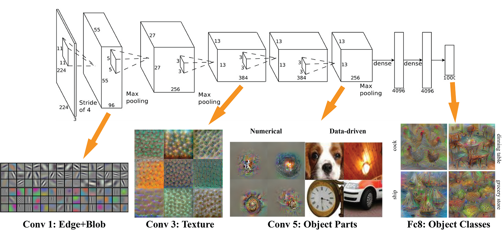
Figure 16: Source [4]

Visualizing Convolutional Neural Networks

In general, the more convolution steps we have, the more complicated features our network will be able to learn to recognize. For example, in Image Classification a ConvNet may learn to detect edges from raw pixels in the first layer, then use the edges to detect simple shapes in the second layer, and then use these shapes to deter higher-level features, such as facial shapes in higher layers [14]. This is demonstrated in Figure 17 below – these features were learnt using a Convolutional Deep Belief Network and the figure is included here just for demonstrating the idea (this is only an example: real life convolution filters may detect objects that have no meaning to humans).
Screen Shot 2016-08-10 at 12.58.30 PM.png
Figure 17: Learned features from a Convolutional Deep Belief Network. Source [21]
Adam Harley created amazing visualizations of a Convolutional Neural Network trained on the MNIST Database of handwritten digits [13]. I highly recommend playing around with it to understand details of how a CNN works.
We will see below how the network works for an input ‘8’. Note that the visualization in Figure 18 does not show the ReLU operation separately.
conv_all.png
Figure 18: Visualizing a ConvNet trained on handwritten digits. Source [13]
The input image contains 1024 pixels (32 x 32 image) and the first Convolution layer (Convolution Layer 1) is formed by convolution of six unique 5 × 5 (stride 1) filters with the input image. As seen, using six different filters produces a feature map of depth six.
Convolutional Layer 1 is followed by Pooling Layer 1 that does 2 × 2 max pooling (with stride 2) separately over the six feature maps in Convolution Layer 1. You can move your mouse pointer over any pixel in the Pooling Layer and observe the 2 x 2 grid it forms in the previous Convolution Layer (demonstrated in Figure 19). You’ll notice that the pixel having the maximum value (the brightest one) in the 2 x 2 grid makes it to the Pooling layer.
Screen Shot 2016-08-06 at 12.45.35 PM.png
Figure 19: Visualizing the Pooling Operation. Source [13]
Pooling Layer 1 is followed by sixteen 5 × 5 (stride 1) convolutional filters that perform the convolution operation. This is followed by Pooling Layer 2 that does 2 × 2 max pooling (with stride 2). These two layers use the same concepts as described above.
We then have three fully-connected (FC) layers. There are:
  • 120 neurons in the first FC layer
  • 100 neurons in the second FC layer
  • 10 neurons in the third FC layer corresponding to the 10 digits – also called the Output layer
Notice how in Figure 20, each of the 10 nodes in the output layer are connected to all 100 nodes in the 2nd Fully Connected layer (hence the name Fully Connected).
Also, note how the only bright node in the Output Layer corresponds to ‘8’ – this means that the network correctly classifies our handwritten digit (brighter node denotes that the output from it is higher, i.e. 8 has the highest probability among all other digits).
final.png
Figure 20: Visualizing the Filly Connected Layers. Source [13]
The 3d version of the same visualization is available here.

Other ConvNet Architectures

Convolutional Neural Networks have been around since early 1990s. We discussed the LeNet above which was one of the very first convolutional neural networks. Some other influential architectures are listed below [3] [4].
  • LeNet (1990s): Already covered in this article.
  • 1990s to 2012: In the years from late 1990s to early 2010s convolutional neural network were in incubation. As more and more data and computing power became available, tasks that convolutional neural networks could tackle became more and more interesting.
  • AlexNet (2012) – In 2012, Alex Krizhevsky (and others) released AlexNet which was a deeper and much wider version of the LeNet and won by a large margin the difficult ImageNet Large Scale Visual Recognition Challenge (ILSVRC) in 2012. It was a significant breakthrough with respect to the previous approaches and the current widespread application of CNNs can be attributed to this work.
  • ZF Net (2013) – The ILSVRC 2013 winner was a Convolutional Network from Matthew Zeiler and Rob Fergus. It became known as the ZFNet (short for Zeiler & Fergus Net). It was an improvement on AlexNet by tweaking the architecture hyperparameters.
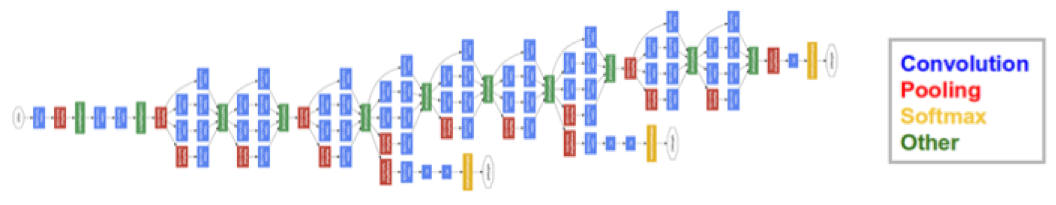
  • GoogLeNet (2014) – The ILSVRC 2014 winner was a Convolutional Network from Szegedy et al. from Google. Its main contribution was the development of an Inception Module that dramatically reduced the number of parameters in the network (4M, compared to AlexNet with 60M).
  • VGGNet (2014) – The runner-up in ILSVRC 2014 was the network that became known as the VGGNet. Its main contribution was in showing that the depth of the network (number of layers) is a critical component for good performance.
  • ResNets (2015) – Residual Network developed by Kaiming He (and others) was the winner of ILSVRC 2015. ResNets are currently by far state of the art Convolutional Neural Network models and are the default choice for using ConvNets in practice (as of May 2016).
  • DenseNet (August 2016) – Recently published by Gao Huang (and others), the Densely Connected Convolutional Network has each layer directly connected to every other layer in a feed-forward fashion. The DenseNet has been shown to obtain significant improvements over previous state-of-the-art architectures on five highly competitive object recognition benchmark tasks. Check out the Torch implementation here.

Conclusion

In this post, I have tried to explain the main concepts behind Convolutional Neural Networks in simple terms. There are several details I have oversimplified / skipped, but hopefully this post gave you some intuition around how they work.
This post was originally inspired from Understanding Convolutional Neural Networks for NLP by Denny Britz (which I would recommend reading) and a number of explanations here are based on that post. For a more thorough understanding of some of these concepts, I would encourage you to go through the notes from Stanford’s course on ConvNets as well as other excellent resources mentioned under References below. If you face any issues understanding any of the above concepts or have questions / suggestions, feel free to leave a comment below.
All images and animations used in this post belong to their respective authors as listed in References section below.

References

  1. karpathy/neuraltalk2: Efficient Image Captioning code in Torch, Examples
  2. Shaoqing Ren, et al, “Faster R-CNN: Towards Real-Time Object Detection with Region Proposal Networks”, 2015, arXiv:1506.01497 
  3. Neural Network Architectures, Eugenio Culurciello’s blog
  4. CS231n Convolutional Neural Networks for Visual Recognition, Stanford
  5. Clarifai / Technology
  6. Machine Learning is Fun! Part 3: Deep Learning and Convolutional Neural Networks
  7. Feature extraction using convolution, Stanford
  8. Wikipedia article on Kernel (image processing) 
  9. Deep Learning Methods for Vision, CVPR 2012 Tutorial 
  10. Neural Networks by Rob Fergus, Machine Learning Summer School 2015
  11. What do the fully connected layers do in CNNs? 
  12. Convolutional Neural Networks, Andrew Gibiansky 
  13. A. W. Harley, “An Interactive Node-Link Visualization of Convolutional Neural Networks,” in ISVC, pages 867-877, 2015 (link). Demo
  14. Understanding Convolutional Neural Networks for NLP
  15. Backpropagation in Convolutional Neural Networks
  16. A Beginner’s Guide To Understanding Convolutional Neural Networks
  17. Vincent Dumoulin, et al, “A guide to convolution arithmetic for deep learning”, 2015, arXiv:1603.07285
  18. What is the difference between deep learning and usual machine learning?
  19. How is a convolutional neural network able to learn invariant features?
  20. A Taxonomy of Deep Convolutional Neural Nets for Computer Vision
  21. Honglak Lee, et al, “Convolutional Deep Belief Networks for Scalable Unsupervised Learning of Hierarchical Representations” (link)