Epilepsyecosystem.org is a crowd-sourcing ecosystem for
improving the performance of seizure prediction algorithms in order to
make seizure prediction a viable treatment option for those suffering
from epilepsy.
Epilepsy afflicts nearly 1% of the world's
population, and is characterized by the occurrence of spontaneous
seizures. For many patients, anticonvulsant medications can be given at
sufficiently high doses to prevent seizures, but patients frequently
suffer side effects. For 20-40% of patients with epilepsy, medications
are not effective. Even after surgical removal of epilepsy, many
patients continue to experience spontaneous seizures. Despite the fact
that seizures occur infrequently, patients with epilepsy experience
persistent anxiety due to the possibility of a seizure occurring. Seizure
forecasting systems have the potential to help patients with epilepsy
lead more normal lives. In order for electrical brain activity (EEG)
based seizure forecasting systems to work effectively, computational
algorithms must reliably identify periods of increased probability of
seizure occurrence. If these seizure-permissive brain states can be
identified, devices designed to warn patients of impeding seizures would
be possible. Patients could avoid potentially dangerous activities like
driving or swimming, and medications could be administered only when
needed to prevent impending seizures, reducing overall side effects. A Crowd-Sourcing Ecosystem for Seizure Prediction
Epilepsyecosystem.org is the evolution of a Crowd-Sourcing Ecosystem for Seizure Prediction that began with the ‘Melbourne-University AES-MathWorks-NIH Seizure Prediction Challenge’
that was hosted on Kaggle.com in 2016. The contest focused on seizure
prediction using long-term electrical brain activity recordings from
humans obtained from the world-first clinical trial of the implantable
NeuroVista Seizure Advisory System. Over 10,000 algorithms were
submitted. The top algorithms from the contest were evaluated on
additional held out data and demonstrated improvements in seizure
prediction performance relative to the original trial results.
Epilepsyecosystem.org offers the opportunity to yield further
improvements with the contest dataset. The top algorithms in the
ecosystem will be invited for evaluation on the full clinical trial
database, a one-of-a-kind world-class dataset, with the aim of finding
the best algorithms for the widest range of patients. Acknowledgments
Epilepsyecosystem.org
is supported by the Aikenhead Centre for Medical Discovery at St.
Vincent’s Hospital Melbourne, the University of Melbourne, Swinburne
University of Technology and Seer Medical. References
Kuhlmann,
L., Karoly, P., Freestone, D.R., Brinkmann, B.H., Temko, A., Barachant,
A., Li, F., Titericz Jr., G., Lang, B.W., Lavery, D., Roman, K.,
Broadhead, D., Dobson, S., Jones, G., Tang, Q., Ivanenko, I., Panichev,
O., Proix, T., Náhlík, M., Grunberg, D.B., Reuben, C., Worrell, G.,
Litt, B., Liley, D.T.J., Grayden, D.B., & Cook, M.J. (2018) Epilepsyecosystem.org: Crowd-Sourcing Reproducible Seizure Prediction with Long-Term Human Intracranial EEG, Brain, awy210, https://doi.org/10.1093/brain/awy210
Kuhlmann,
L., Lehnertz, K., Richardson, M., Schelter, B., & Zaveri, H. (2018)
Seizure prediction — ready for a new era. Nature Reviews Neurology. In
Press (accepted 13/07/2018).
Freestone, D. R., Karoly, P. J.,
Peterson, A. D., Kuhlmann, L., Lai, A., Goodarzy, F., & Cook, M. J.
(2015). Seizure prediction: science fiction or soon to become reality?. Current neurology and neuroscience reports, 15(11), 73.
Karoly,
P. J., Ung, H., Grayden, D. B., Kuhlmann, L., Leyde, K., Cook, M. J.,
& Freestone, D. R. (2017). The circadian profile of epilepsy
improves seizure forecasting. Brain, 140(8), 2169-2182.
Cook
MJ, O'Brien TJ, Berkovic SF, Murphy M, Morokoff A, Fabinyi G, D'Souza
W, Yerra R, Archer J, Litewka L, Hosking S, Lightfoot P, Ruedebusch V,
Sheffield WD, Snyder D, Leyde K, Himes D (2013) Prediction of seizure
likelihood with a long-term, implanted seizure advisory system in
patients with drug-resistant epilepsy: a first-in-man study. Lancet
Neurology 12:563-571.
Brinkmann, B. H., Wagenaar, J., Abbot, D.,
Adkins, P., Bosshard, S. C., Chen, M., ... & Pardo, J. (2016).
Crowdsourcing reproducible seizure forecasting in human and canine
epilepsy. Brain, 139(6), 1713-1722.
Gadhoumi, K., Lina, J. M.,
Mormann, F., & Gotman, J. (2016). Seizure prediction for therapeutic
devices: A review. Journal of neuroscience methods, 260, 270-282.
Andrzejak RG, Chicharro D, Elger CE, Mormann F (2009) Seizure prediction: Any better than chance? Clin Neurophysiol.
Mormann F, Andrzejak RG, Elger CE, Lehnertz K (2007) Seizure pre
The purpose of this repository is not to implement machine learning algorithms by using 3rd party library "one-liners" but
rather to practice implementing these algorithms from scratch and get
better understanding of the mathematics behind each algorithm. That's
why all algorithms implementations are called "homemade" and not
intended to be used for production.
Important paper from Google on large batch optimization. They do
impressively careful experiments measuring # iterations needed to
achieve target validation error at various batch sizes. The main
"surprise" is the lack of surprises. [thread]
VER THE past five years researchers in artificial intelligence have become the rock stars of the technology world. A branch of AI known as deep learning, which uses neural networks to churn through large volumes of data looking for patterns, has proven so useful that skilled practitioners can command high six-figure salaries to build software for Amazon, Apple, Facebook and Google. The top names can earn over $1m a year.
The standard route into these jobs has been a PhD in computer science from one of America’s elite universities. Earning one takes years and requires a disposition suited to academia, which is rare among more normal folk. Graduate students are regularly lured away from their studies by lucrative jobs.
That is changing. This month fast.ai, an education non-profit based in San Francisco, kicked off the third year of its course in deep learning. Since its inception it has attracted more than 100,000 students, scattered around the globe from India to Nigeria. The course and others like it come with a simple proposition: there is no need to spend years obtaining a PhD in order to practise deep learning. Creating software that learns can be taught as a craft, not as a high intellectual pursuit to be undertaken only in an ivory tower. Fast.ai’s course can be completed in just seven weeks.
Demystifying the subject, to make it accessible to anyone who wants to learn how to build AI software, is the aim of Jeremy Howard, who founded fast.ai with Rachel Thomas, a mathematician. He says school mathematics is sufficient. “No. Greek. Letters,” Mr Howard intones, thumping the table for punctuation.
It is working. A graduate from fast.ai’s first year, Sara Hooker, was hired into Google’s highly competitive AI residency programme after finishing the course, having never worked on deep learning before. She is now a founding member of Google’s new AI research office in Accra, Ghana, the firm’s first in Africa. In Bangalore, some 2,400 people are members of AI Saturdays, which follows the course together as a gigantic study group. Andrei Karpathy, one of deep learning’s foremost practitioners, recommends the course.
Fast.ai’s is not the only alternative AI programme. AI4ALL, another non-profit venture, works to bring AI education to schoolchildren in the United States that would otherwise not have access to it. Andrew Ng, another well-known figure in the field, has started his own online course, deeplearning.ai.
Mr Howard’s ambitions run deeper than loosening the AI labour market. His aim is to spread deep learning into many hands, so that it may be applied in as diverse a set of fields by as diverse a group of people as possible. So far, it has been controlled by a small number of mostly young white men, almost all of whom have been employed by the tech giants. The ambition, says Mr Howard, is for AI training software to become as easy to use and ubiquitous as sending an email on a smartphone.
Some experts worry that this will serve only to create a flood of dodgy AI systems which will be useless at best and dangerous at worst. An analogy may allay those concerns. In the earliest days of the internet, only a select few nerds with specific skills could build applications. Not many people used them. Then the invention of the world wide web led to an explosion of web pages, both good and bad. But it was only by opening up to all that the internet gave birth to online shopping, instant global communications and search. If Mr Howard and others have their way, making the development of AI software easier will bring forth a new crop of fruit of a different kind. This article appeared in the Business section of the print edition under the headline "Learning, fast and deep"
ESP-WHO is a face detection and recognition platform that is currently based on Espressif Systems' ESP32 chip. ESP-WHO is within Espressif Systems AI framework, with the focus on face detection and recognition so far.
Everyone is talking about Artificial Intelligence,
but what’s really going on? Is AI going to solve all your problems? And
what even IS AI? What are the key things you need to take into account
when building AI solutions? In practice AI is often used as an umbrella
term, and most of the solutions we refer to are Machine Learning – and
it has been around for some time. For example, the first artificial
neural networks emerged in the mid 1900s.
Sure, methods and algorithms have evolved a lot, and perhaps even
more significantly computing power has increased drastically, but we
have been using and developing machine learning models for quite some
time. Even though there have been fantastic recent advances in ease of
use through ready toolkits like TensorFlow or manged cloud services like Sagemaker,
I do think many of the fundamental things learned through experience
over the years still apply, but have sometimes seen some of the
fundamentals can get forgotten in all the excitement. I have been
working in the field for a while now, and just wanted to share a few
principles that I think everyone should keep in mind when designing and
building – or evaluating, if you are sitting on that side of the fence –
successful AI/ML solutions.
Raster Vision is an open source framework for Python developers
building computer vision models on satellite, aerial, and other large
imagery sets, including non-georeferenced data like oblique drone
imagery. It allows engineers to quickly and repeatably configure
experiments that go through core components of a machine learning
workflow: analyzing training data, creating training chips, training
models, creating predictions, evaluating models, and bundling the model
files and configuration for easy deployment.
The input to a Raster Vision workflow is a set of images and training
data, optionally with Areas of Interest (AOIs), that describe where the
images are labeled. Running a workflow results in evaluation metrics
and a packaged model and configuration that enables easy deployment.
Raster Vision also supports running multiple experiments at once to find
the best model (or models) to deploy.
Win a trip around the world based on an algorithm you write!
This is your chance to get your hands on something that’s normally
purely theoretical and have some fun with it. The Travelling Salesman
Challenge is returning for 2018, and this time you’re finding the
cheapest route between whole areas.
Artificial intelligence — and its subfield of machine learning — is reshaping the landscape of news and information. From the algorithms filtering what we see on social media, to the use of machine learning to generate news stories and online content, AI has and will continue to play a major role in shaping what and how information is distributed and consumed.
As researchers and companies continue to advance the technical state of the art, we believe that it is necessary to ensure that AI serves the public good. This means not only working to address the problems presented by existing AI systems, but articulating what realistic, better alternatives might look like.
This open challenge, which will award up to $750,000 to a range of projects, is seeking fresh and experimental approaches to four specific problems at the intersection of AI and the news:
Governing the Platforms: Ensuring that AI serves the public good requires the public to know how the platforms are deploying these technologies and how they shape the flow of information through the web today. However, as many others have pointed out, the level of transparency and accountability around these decisions has been limited, and we’re seeking ideas that help to raise it. This might be new policies in the form of draft legislation, or technical tools that help keep an eye on the information ecosystem.
Stopping Bad Actors: AI might be applied by a variety of actors to spread disinformation, from powering believable bots on social media to fabricating realistic video and audio. This exacerbates a range of existing problems in news and information. We’re seeking approaches we can take to detect and counter this next generation of propaganda.
Empowering Journalism: Journalists play a major role in shaping public understanding of AI, its impact on the information ecosystem, and what we should do to ensure the technology is used ethically. But it can be hard to keep up with the latest developments in the technical research and communicate them effectively to society at large. We’re seeking ideas that will help bolster this community in this important work, and give them the tools they need to effectively communicate about AI and its impact.
Reimagining AI and News: It is easy to find a lot of things to critique about the influence that automation and AI have on the news and information space. More challenging is articulating plausible alternatives for how these platforms should be designed and how they should deploy these technologies. We’re interested in ideas that paint a picture of the future: How might platforms from smartphones and social media sites to search engines and online news outlets be redesigned in part or entirely to better serve the public good?
We believe there are a diverse range of communities that can bring their expertise to bear on these issues but are frequently left out of the conversation. This challenge is open to anyone: We’re looking for journalists, designers, technologists, activists, entrepreneurs, artists, lawyers from a variety of communities around the world — anyone who thinks they have a good idea about addressing these problems that may not have been tried before.
Decades-old discoveries are now electrifying the computing industry and will soon transform corporate America.
Over the past four years, readers have doubtlessly noticed quantum
leaps in the quality of a wide range of everyday technologies.
Most obviously, the speech-recognition functions on our smartphones
work much better than they used to. When we use a voice command to call
our spouses, we reach them now. We aren’t connected to Amtrak or an
angry ex.
In fact, we are increasingly interacting with our computers by just
talking to them, whether it’s Amazon’s Alexa, Apple’s Siri, Microsoft’s
Cortana, or the many voice-responsive features of Google. Chinese search
giant Baidu says customers have tripled their use of its speech
interfaces in the past 18 months.
Machine translation and other forms of language processing have also become far more convincing, with GoogleGOOGL0.92%
, MicrosoftMSFT0.38%
, FacebookFB1.13%
, and Baidu BIDU0.35%
unveiling new tricks every month. Google Translate now
renders spoken sentences in one language into spoken sentences in
another for 32 pairs of languages, while offering text translations for
103 tongues, including Cebuano, Igbo, and Zulu. Google’s Inbox app
offers three ready-made replies for many incoming emails.
Helpful installation and setup instructions can be found in the README.md file of Chapter 1
To access the code materials for a given chapter, simply click on the open dir links next to the chapter headlines to navigate to the chapter subdirectories located in the code/ subdirectory. You can also click on the ipynb links below to open and view the Jupyter notebook of each chapter directly on GitHub.
In addition, the code/
subdirectories also contain .py script files, which were created from
the Jupyter Notebooks. However, I highly recommend working with the
Jupyter notebook if possible in your computing environment. Not only do
the Jupyter notebooks contain the images and section headings for easier
navigation, but they also allow for a stepwise execution of individual
code snippets, which -- in my opinion -- provide a better learning
experience. Please note that these are just the code examples
accompanying the book, which I uploaded for your convenience; be aware
that these notebooks may not be useful without the formulae and
descriptive text.
Machine Learning - Giving Computers the Ability to Learn from Data [open dir] [ipynb]
Training Machine Learning Algorithms for Classification [open dir] [ipynb]
A Tour of Machine Learning Classifiers Using Scikit-Learn [open dir] [ipynb]
Building Good Training Sets – Data Pre-Processing [open dir] [ipynb]
Compressing Data via Dimensionality Reduction [open dir] [ipynb]
Learning Best Practices for Model Evaluation and Hyperparameter Optimization [open dir] [ipynb]
Combining Different Models for Ensemble Learning [open dir] [ipynb]
Applying Machine Learning to Sentiment Analysis [open dir] [ipynb]
Embedding a Machine Learning Model into a Web Application [open dir] [ipynb]
Predicting Continuous Target Variables with Regression Analysis [open dir] [ipynb]
Working with Unlabeled Data – Clustering Analysis [open dir] [ipynb]
Implementing a Multi-layer Artificial Neural Network from Scratch [open dir] [ipynb]
Parallelizing Neural Network Training with TensorFlow [open dir] [ipynb]
Going Deeper: The Mechanics of TensorFlow [open dir] [ipynb]
Classifying Images with Deep Convolutional Neural Networks [open dir] [ipynb]
Modeling Sequential Data Using Recurrent Neural Networks [open dir] [ipynb]
mlcourse.ai is an open
Machine Learning course by OpenDataScience. The course is designed to
perfectly balance theory and practice; therefore, each topic is followed
by an assignment with a deadline in a week. You can also take part in
several Kaggle Inclass competitions held during the course and work on
your own projects.
Next session starts on October 1, 2018. Fill in this form to participate.
Navigation:
Prerequisites. Our
course is not for total newbies. Though Machine Learning is covered
from scratch, still participants are expected to know some math and be
able to write code in Python.
Assignments. Here you’ll find demo versions of assignments. Assignments in a new session of the course will be different.
News. Here you can track main announcements during the course.
Resources. Links to other information mirrors of this course like Medium stories, Kaggle Kernels etc.
Contacts. Ways of reaching OpenDataScience and course team.
https://blog.floydhub.com/ten-a-from-fast-ai/
Right now, Jeremy Howard – the co-founder of fast.ai – currently holds the 105th highest score for the plant seedling classification contest
on Kaggle, but he's dropping fast. Why? His own students are beating
him. And their names can now be found across the tops of leaderboards
all over Kaggle. When I left you I was but the learner, but now I am the master.So
what are these secrets that are allowing novices to implement
world-class algorithms in mere weeks, leaving behind experienced deep
learning practitioners in their GPU-powered wake? Allow me to tell you
in ten simple steps.
Read on if you're already practicing
deep learning and want to quickly get an overview of the powerful
techniques that fast.ai uses in their courses. Read on if you've already
completed fast.ai and want to recap some of what you were supposed to
have already learned. Read on if you're flirting with the idea of
studying deep learning, and would like to see how the field is evolving
and what fast.ai can offer beginners.
Now, before we
begin, you should know that you'll need access to GPUs to run fast.ai
content effectively. For my fast.ai projects, I've been using FloydHub.
After much experimentation and research with other cloud-based
solutions, I've found FloydHub is the best and easiest way to train deep
learning models on cloud GPUs. I love being able to easily keep track
of my experiments in Projects
on FloydHub, making it especially easy to visualize and filter which
models are performing best. They also have the simplest solution for
managing (and automatically versioning) your datasets, which you'll
learn is going to be super valuable down the road in any DL project.
Okay, let's get started.
1. Use the Fast.ai library
from fast.ai import *
The
fast.ai library is not only a toolkit to get newbies quickly
implementing deep learning, but a powerful and convenient source of
current best practices. Each time the fast.ai team (and their network of
AI researchers & collaborators) finds a particularly interesting
paper, they test it out on a variety of datasets and work out how to
tune it. If they are successful, it gets implemented in the library, and
the technology can be quickly accessed by its users.
The result
is a powerful toolbox, including quick access to best-current practices
such as stochastic gradient descent with restarts, differential learning
rates, and test-time augmentation (not to mention many more).
Each
of these techniques will be described below, and we will show how you
can rapidly implement them using the fast.ai library. The library is
built upon PyTorch, and you can use them together quite fluidly.To get going with the library on FloydHub, check out their 2-min installation.
2. Don’t use one learning rate, use many
Differential
Learning rates mean higher layers change more than deeper layers during
training. Building deep learning models on top of pre-existing
architectures is a proven method to generate much better results in
computer vision tasks. Most of these architectures (i.e. Resnet, VGG,
inception…) are trained on ImageNet, and depending on the similarity of
your data to the images on ImageNet, these weights will need to be
altered more or less greatly. When it comes to modifying these weights,
the last layers of the model will often need the most changing, while
deeper levels that are already well trained to detecting basic features
(such as edges and outlines) will need less.
So firstly, to get a pre-trained model with the fast ai library use the following code:
from fastai.conv_learner import *

# import library for creating learning object for convolutional #networks
model = VVG16()

# assign model to resnet, vgg, or even your own custom model
PATH = './folder_containing_images'
data = ImageClassifierData.from_paths(PATH)

# create fast ai data object, in this method we use from_paths where
# inside PATH each image class is separated into different folders

learn = ConvLearner.pretrained(model, data, precompute=True)

# create a learn object to quickly utilise state of the art
# techniques from the fast ai library
With the learn
object now created, we can solve the problem of only finely tuning the
last layers by quickly freezing the first layers:
learn.freeze()

# freeze layers up to the last one, so weights will not be updated.

learning_rate = 0.1
learn.fit(learning_rate, epochs=3)

# train only the last layer for a few epochs
Once the
last layers are producing good results, we implement differential
learning rates to alter the lower layers as well. The lower layers want
to be altered less, so it is good practice to set each learning rate to
be 10 times lower than the last:
learn.unfreeze()

# set requires_grads to be True for all layers, so they can be updated

learning_rate = [0.001, 0.01, 0.1]
# learning rate is set so that deepest third of layers have a rate of 0.001, # middle layers have a rate of 0.01, and final layers 0.1.

learn.fit(learning_rate, epochs=3)
# train model for three epoch with using differential learning rates
3. How to find the right learning rate
The
learning rate is the most important hyper-parameter for training neural
networks, yet until recently deciding its value has been incredibly
hacky. Leslie Smith may have stumbled upon the answer in his paper on cyclical learning rates; a relatively unknown discovery until it was promoted by the fast.ai course.
In
this method, we do a trial run and train the neural network using a low
learning rate, but increase it exponentially with each batch. This can
be done with the following code:
learn.lr_find()
# run on learn object where learning rate is increased  exponentially

learn.sched.plot_lr()
# plot graph of learning rate against iterations
The learning rate is increased exponentially with every iterationMeanwhile, the loss is recorded for every value of the learning rate. We then plot loss against learning rate:
learn.sched.plot()
# plots the loss against the learning rate
Find where the loss is still decreasing but has not plateaued.The
optimum learning rate is determined by finding the value where the
learning rate is highest and the loss is still descending, in the above
case about this value would be 0.01.
4. Cosine annealing
With
each batch of stochastic gradient descent (SGD), your network should be
getting closer and closer to a global minimum value for the loss. As it
gets closer to this minimum, it hence makes sense that the learning
rate should get smaller so that your algorithm does not overshoot, and
instead settles as close to this point as possible. Cosine annealing
solves this problem by decreasing the learning rate following the cosine
function as seen in the figure below. As we increase x, we see cosine(x) decrease following this wavy shape.Looking
at the figure above, we see that as we increase x the cosine value
descends slowly at first, then more quickly and then slightly slower
again. This mode of decreasing works well with the learning rate,
yielding great results in a computationally efficient manner.
learn.fit(0.1, 1)
# Calling learn fit automatically takes advantage of cosine annealing
The technique is implemented automatically by the fast ai library when using learn.fit(). The above code would have our learning rate decrease across the epoch as shown in the figure below. Learning rate decreases across an epoch that takes 200 iterations However we can go one step further than this even, and introduce restarts
5. Stochastic Gradient Descent with restarts
During training it is possible for gradient descent to get stuck at local minima rather than the global minimum. Gradient descent can get stuck at local minimaBy
increasing the learning rate suddenly, gradient descent may “hop” out
of the local minima and find its way toward the global minimum. Doing
this is called stochastic gradient descent with restarts (SGDR), an idea
shown to be highly effective in a paper by Loshchilov and Hutter.
SGDR is also handled for you automatically by the fast ai library. When calling learn.fit(learning_rate, epochs),
the learning rate is reset at the start of each epoch to the original
value you entered as a parameter, then decreases again over the epoch as
described above in cosine annealing. The learning rate is restored to its original value after each epoch.Each time the learning rate drops to it’s minimum point (every 100 iterations in the figure above), we call this a cycle.
cycle_len = 1
# decide how many epochs it takes for the learning rate to fall to
# its minimum point. In this case, 1 epoch

cycle_mult=2
# at the end of each cycle, multiply the cycle_len value by 2

learn.fit(0.1, 3, cycle_len=2, cycle_mult=2)
# in this case there will be three restarts. The first time with
# cycle_len of 1, so it will take 1 epoch to complete the cycle.
# cycle_mult=2 so the next cycle with have a length of two epochs,
# and the next four.
Each cycle taking twice as many epochs to complete as the prior cyclePlaying
around with these parameters, along with using differential learning
rates, are the key techniques allowing fast ai users to perform so well
on image classification problems. Cycle_mult and cycle_len are discussed here on the fast.ai forum, while the concepts above regarding learning rate can be found explained more fully in this fast ai lesson and this blog post.
6. Anthropomorphise your activation functions
Softmax
likes to pick just one thing. Sigmoid wants to know where you are
between -1 and 1, and beyond these values won’t care how much you
increase. Relu is a club bouncer who won’t let negative numbers through
the door.
It may seem silly to treat activation functions in such a
manner, but giving them a character ensures not using them for the
wrong task. As Jeremy Howard points out, even academic papers often use
softmax for multi-class classification, and I too have already seen it
used incorrectly in blogs and papers during my short time studying DL.
7. Transfer learning is hugely effective in NLP
Just
as using pre-trained models has proven immensely effective in computer
vision, it is becoming increasingly clear that natural language
processing (NLP) models can benefit from doing the same.
In the 4th lesson
of fast.ai, Jeremy Howard builds a model to determine if IMDB reviews
are positive or negative using transfer learning. The power of this
technique is observed instantly, where the accuracy he achieves beat all
previous efforts of the time presented in a paper by Bradbury et al. Pre-existing architectures deliver state of the art NLP results.The
secret to success lies in training a model firstly to gain some
understanding of the language, before using this pre-trained model as a
part of a model to analyze sentiment.
To create the first model, a
recurrent neural network (RNN) is trained to predict the next word in a
sequence of text. This is known as language modeling. Once the network
is trained to a high degree of accuracy, its encodings for each word are
passed on to a new model that is used for sentiment analysis.
In
the example we see this language model being integrated with a model to
perform sentiment analysis, but this same method could be used for any
NLP task from translation to data extraction.
And again the same
principles as above in computer vision apply here, where freezing and
using differential learning rates can yield better results.
The
implementation of this method for NLP is too detailed for me to share
the code in this post, but if you are interested watch the lesson here and access the code here.
8. Deep learning can challenge ML in tackling structured data
Fast.ai
shows techniques to rapidly generate great results on structured data
without having to resort to feature engineering or apply domain specific
knowledge.
Their library makes the most of PyTorch’s embedding
functions, allowing rapid conversion of categorical variables into
embedding matrixes.
The technique they show is relatively
straight forward, and simply involves turning the categorical variables
into numbers and then assigning each value an embedding vector: Each day of the week is given an embedding with four values.The
advantage of doing this compared to the traditional approach of
creating dummy variables (i.e. doing one hot encodings), is that each
day can be represented by four numbers instead of one, hence we gain
higher dimensionality and much richer relationships.
The implementation shown in this lesson (the code here) gained third place in the Rossman Kaggle competition, only beaten by domain experts who had their own code to create many, many extra features.
The
idea that using deep learning dramatically reduces need for feature
engineering has been confirmed by Pinterest too, who have said this to
be the case ever since they switched to deep learning models, gaining
state of the art results with a lot less work!
9. A game-winning bundle: building up sizes, dropout and TTA
On
the 30th April, the fast.ai team won the DAWNBench competition (run by
Stanford University) on Imagenet and CIFAR10 classification. In Jeremy’s write-up of the victory, he credits their success to the little extra touches available in the fast.ai library.
One of these is the concept of Dropout, proposed by Geoffrey Hinton two years ago in this seminal paper.
Despite its initial popularity, it seems to be somewhat ignored in
recent computer vision papers. However, PyTorch has made its
implementation incredibly easy, and with fast ai on top it’s easier than
ever. Blank spaces represent activations knocked out by dropout function.Dropout
combats overfitting and so would have proved crucial in winning on a
relatively small dataset such at CIFAR10. Dropout is implemented
automatically by fast ai when creating a learn object, though can be
altered using the ps variable as shown here:
learn = ConvLearner.pretrained(model, data, ps=0.5, precompute=True)
# creates a dropout of 0.5 (i.e. half the activations) on test dataset.
# This is automatically turned off for the validation set
For more information on dropout see this video (from 4:57).
Another
incredibly simple and effective method they used for tackling
overfitting and improving accuracy is training on smaller image sizes,
then increasing the size and training the same model on them again.
# create a data object with images of sz * sz pixels
def get_data(sz):
	tmfs = tfms_from_model(model, sz)
	# tells what size images should be, additional transformations such
	# image flips and zooms can easily be added here too

	data = ImageClassifierData.from_paths(PATH, tfms=tfms)
	# creates fastai data object of create size

	return data

learn.set_data(get_data(299))
# changes the data in the learn object to be images of size 299
# without changing the model.

learn.fit(0.1, 3)
# train for a few epochs on larger versions of images, avoiding overfitting
A
final technique that can raise accuracy by one percent or two is test
time augmentation (TTA). This involves taking a series of different
versions of the original image (for example cropping different areas, or
changing the zoom) and passing them through the model. The average
output is then calculated for the different versions and this is given
as the final output score for the image. It can be called by running learn.TTA().
preds, target = learn.TTA()
This
technique is effective as perhaps the original cropping of an image may
miss out a vital feature. Providing the model with multiple versions of
the picture and taking an average makes this less likely to have an
effect.
10. Creativity is key
Not
only did the fast.ai team win prizes for fastest speed in the DAWNBench
competition, but these same algorithms also won the prize for being
cheapest to run. The lesson to be learnt here is that creating
successful DL applications is not just a case of chucking huge amounts
of GPU at the issue, but should instead be a question of creativity, of
intuition and innovation.
Most of the breakthroughs discussed in
this article (dropout, cosine annealing, SGD with restarts, the list
goes on…) in fact were such exact moments, where someone thought of
approaching the problem differently. These approaches then brought
increases in accuracy greater than those that would have been achieved
by simply throwing another thousand images at the problem with a handful
of IBM computers.
So just because there are a lot of big dogs out
there with a lot of big GPUs in Silicon Valley, don’t think that you
can’t challenge them, or that you can’t create something special or
innovative.
In fact, perhaps sometimes you can see constraints as a blessing; after all, necessity is the mother of invention.
About Samuel Lynn-Evans
For
the last 10 years, Sam has combined his passion for science and
languages by teaching life sciences in foreign countries. Seeing the
huge potential for ML in scientific progress, he began studying AI at
school 42 in Paris, with the aim of applying NLP to biological and
medical problems.
You can follow along with Sam on Twitter and Medium.
Neural networks trained to classify images have a remarkable — and surprising! — capacity to generate images.
Techniques such as DeepDream
[1]
, style transfer
[2]
, and feature visualization
[3]
leverage this capacity as a powerful tool for exploring the
inner workings of neural networks, and to fuel a small artistic movement
based on neural art.
All these techniques work in roughly the same way.
Neural networks used in computer vision have a rich internal
representation of the images they look at.
We can use this representation to describe the properties we want an
image to have (e.g. style), and then optimize the input image to have
those properties.
This kind of optimization is possible because the networks are
differentiable with respect to their inputs: we can slightly tweak the
image to better fit the desired properties, and then iteratively apply
such tweaks in gradient descent.
Typically, we parameterize the input image as the RGB values of each
pixel, but that isn’t the only way.
As long as the mapping from parameters to images is differentiable,
we can still optimize alternative parameterizations with gradient
descent.
This blog shares some brief thoughts on machine learning accuracy and bias.
Let’s start with some comments about a recent ACLU blog in
which they run a facial recognition trial. Using Rekognition, the ACLU
built a face database using 25,000 publicly available arrest photos and
then performed facial similarity searches of that database using public
photos of all current members of Congress. They found 28 incorrect
matches out of 535, using an 80% confidence level; this is a 5%
misidentification (sometimes called ‘false positive’) rate and a 95%
accuracy rate. The ACLU has not published its data set, methodology, or
results in detail, so we can only go on what they’ve publicly said. But,
here are some thoughts on their claims:
The default confidence threshold for facial recognition APIs
in Rekognition is 80%, which is good for a broad set of general use
cases (such as identifying celebrities on social media or family members
who look alike in a photos app), but it’s not the right one for public
safety use cases. The 80% confidence threshold used by the ACLU is far
too low to ensure the accurate identification of individuals; we would
expect to see false positives at this level of confidence. We recommend
99% for use cases where highly accurate face similarity matches are
important (as indicated in our public documentation).
1. To illustrate the impact of confidence threshold on false
positives, we ran a test where we created a face collection using a
dataset of over 850,000 faces commonly used in academia. We then used
public photos of all members of US Congress (the Senate and House) to
search against this collection in a similar way to the ACLU blog.
When we set the confidence threshold at 99% (as we recommend
in our documentation), our misidentification rate dropped to 0% despite
the fact that we are comparing against a larger corpus of faces (30x
larger than ACLU’s tests). This illustrates how important it is for
those using technology to help with public safety issues to pick
appropriate confidence levels, so they have few (if any) false
positives.
2. In real-world public safety and law enforcement scenarios,
Amazon Rekognition is almost exclusively used to help narrow the field
and allow humans to expeditiously review and consider options using
their judgment (and not to make fully autonomous decisions), where it
can help find lost children, fight against human trafficking, or prevent
crimes. Rekognition is generally only the first step in identifying an
individual. In other use cases (such as social media), there isn’t the
same need to double check so that confidence thresholds can be lower.
3. In addition to setting the confidence threshold far too
low, the Rekognition results can be significantly skewed by using a
facial database that is not appropriately representative that is itself
skewed. In this case, ACLU used a facial database of mugshots that may
have had a material impact on the accuracy of Rekognition findings.
4. The advantage of a cloud-based machine learning application
like Rekognition is that it is constantly improving as we continue to
improve the algorithm with more data. Our customers immediately get the
benefit of those improvements. We continue to focus on our mission of
making Rekognition the most accurate and powerful tool for identifying
people, objects, and scenes – and that certainly includes ensuring that
the results are free of any bias that impacts accuracy. We’ve been able
to add a lot of value for customers and the world at large already with
Rekognition in the fight against human trafficking, reuniting lost
children with their families, reducing fraud for mobile payments, and
improving security, and we’re excited about continuing to help our
customers and society at large with Rekognition in the future.
5. There is a general misconception that people can match
faces to photos better than machines. In fact, the National Institute
for Standards and Technology (“NIST”) recently shared a study of facial
recognition technologies that are at least two years behind the state of
the art used in Rekognition and concluded that even those older
technologies can outperform human facial recognition abilities.
A final word about the misinterpreted ACLU results. When there
are new technological advances, we all have to clearly understand
what’s real and what’s not. There’s a difference between using machine
learning to identify a food object and using machine learning to
determine whether a face match should warrant considering any law
enforcement action. The latter is serious business and requires much
higher confidence levels. We continue to recommend that customers do not
use less than 99% confidence levels for law enforcement matches, and
then to only use the matches as one input across others that make sense
for each agency. But, machine learning is a very valuable tool to help
law enforcement agencies, and while being concerned it’s applied
correctly, we should not throw away the oven because the temperature
could be set wrong and burn the pizza. It is a very reasonable idea,
however, for the government to weigh in and specify what temperature (or
confidence levels) it wants law enforcement agencies to meet to assist
in their public safety work.
You may be interested in my new arXiv paper,
joint work with Xi Cheng, an undergraduate at UC Davis (now heading to
Cornell for grad school); Bohdan Khomtchouk, a post doc in biology at
Stanford; and Pete Mohanty, a Science, Engineering
& Education Fellow in statistics at Stanford. The paper is of a
provocative nature, and we welcome feedback.
A summary of the paper is:
We present a very simple, informal mathematical argument that neural
networks (NNs) are in essence polynomial regression (PR). We refer to
this as NNAEPR.
NNAEPR implies that we can use our knowledge of the “old-fashioned”
method of PR to gain insight into how NNs — widely viewed somewhat
warily as a “black box” — work inside.
One such insight is that the outputs of an NN layer will be prone to
multicollinearity, with the problem becoming worse with each successive
layer. This in turn may explain why convergence issues often develop in
NNs. It also suggests that NN users tend to use overly large networks.
NNAEPR suggests that one may abandon using NNs altogether, and simply use PR instead.
We investigated this on a wide variety of datasets, and found that in every case PR did as well as, and often better than, NNs.
We have developed a feature-rich R package, polyreg, to facilitate using PR in multivariate settings.
Much work remains to be done (see paper), but our results so far are
very encouraging. By using PR, one can avoid the headaches of NN, such
as selecting good combinations of tuning parameters, dealing with
convergence problems, and so on.
Also available are the slides for our presentation at GRAIL on this project.
Understand the Concepts, Techniques and Mathematical Frameworks Used by Experts in Machine Learning
About This Course
Bloomberg presents "Foundations of Machine Learning," a
training course that was initially delivered internally to the company's
software engineers as part of its "Machine Learning EDU" initiative.
This course covers a wide variety of topics in machine learning and
statistical modeling. The primary goal of the class is to help
participants gain a deep understanding of the concepts, techniques and
mathematical frameworks used by experts in machine learning. It is
designed to make valuable machine learning skills more accessible to
individuals with a strong math background, including software
developers, experimental scientists, engineers and financial
professionals.
The 30 lectures in the course are embedded below, but may also be viewed in this YouTube playlist.
The course includes a complete set of homework assignments, each
containing a theoretical element and implementation challenge with
support code in Python, which is rapidly becoming the prevailing
programming language for data science and machine learning in both
academia and industry. This course also serves as a foundation on which
more specialized courses and further independent study can build.
Check back soon for how to register for our Piazza discussion board. Common questions from previous editions of the course are posted in our FAQ.
The first lecture, Black Box Machine Learning, gives a quick start introduction to practical machine learning and only requires familiarity with basic programming concepts.
Prerequisites
The quickest way to see if the mathematics level of the course is for you is to take a look at this mathematics assessment, which is a preview of some of the math concepts that show up in the first part of the course.
Solid mathematical background,
equivalent to a 1-semester undergraduate course in each of the
following: linear algebra, multivariate differential calculus,
probability theory, and statistics. The content of NYU's DS-GA-1002: Statistical and Mathematical Methods would be more than sufficient, for example.
Python programming required for most homework assignments.
Recommended: At least one advanced, proof-based mathematics course
Recommended: Computer science background up to a "data structures and algorithms" course
Deep
reinforcement learning has rapidly become one of the hottest research
areas in the deep learning ecosystem. The fascination with reinforcement
learning is related to the fact that, from all the deep learning
modalities, is the one that resemble the most how humans learn. In the
last few years, no company in the world has done more to advance the
stage of deep reinforcement learning than Alphabet’s subsidiary
DeepMind.
Since
the launch of its famous AlphaGo agent, DeepMind has been at the
forefront of reinforcement learning research. A few days ago, they published a new research that attempts to tackle one of the most challenging aspects of reinforcement learning solutions: multi-tasking.
Since
we are infants, multi-tasking becomes an intrinsic element of our
cognition. The ability to performing and learning similar tasks
concurrently is essential to the development of the human mind. From the
neuroscientific standpoint, multi-tasking remains largely a mystery and
that, not surprisingly, we have had a heck of hard time implementing
artificial intelligence(AI) agents that can efficiently learn multiple
domains without requiring a disproportional amount of resources. This
challenge is even more evident in the case of deep reinforcement
learning models that are based on trial and error exercises which can
easily cross the boundaries of a single domain. Biologically speaking,
you can argue that all learning is a multi-tasking exercise.
Let’s
take a classic deep reinforcement learning scenario such as
self-driving vehicles. In that scenarios, AI agents need to concurrently
learn different aspects such as distance, memory or navigation while
operating under rapidly changing parameters such as vision quality or
speed. Most reinforcement learning methods today are focused on learning
a single task and the models that track multi-task learning are too
difficult to scale to be practical.
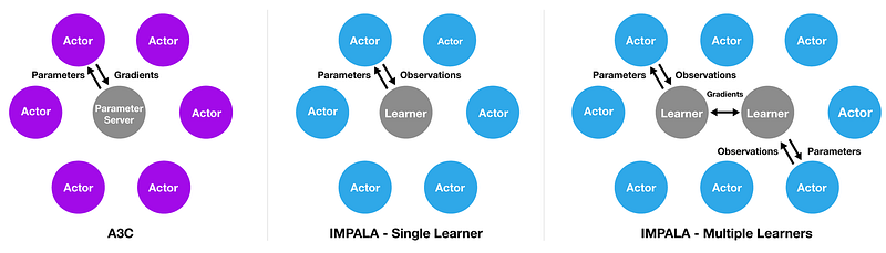
In
their recent research the DeepMind team proposed a new architecture for
deep reinforcement multi-task learning called Importance Weighted
Actor-Learner Architecture (IMPALA). Inspired by another popular
reinforcement learning architecture called A3C,
IMPALA leverages a topology of different actors and learners that can
collaborate to build knowledge across different domains. Traditionally,
deep reinforcement learning models use an architecture based on a single
learner combined with multiple actors. In that model, the Each actor
generates trajectories and sends them via a queue to the learner. Before
starting the next trajectory, actor retrieves the latest policy
parameters from learner. IMPALA uses an architecture that collect
experience which is passed to a central learner that computes gradients,
resulting in a model that has completely independent actors and
learners. This simple architecture enables the learner(s) to be
accelerated using GPUs and actors to be easily distributed across many
machines.
In
addition to the multi-actor architecture model, the IMPALA research
also introduces a new algorithm called V-Trace that focuses off-policy
learning. The idea of V-Trace is to mitigate the lag between when
actions are generated by the actors and when the learner estimates the
gradient.
The DeepMind team tested IMPALA on different scenarios using its famous DMLab-30
training set and the results were impressive. IMPALA proved to achieve
better performance compared to A3C variants in terms of data efficiency,
stability and final performance. This might be the first deep
reinforcement learning models that has been able to efficiently operate
in multi-task environments.
The Places dataset is designed following principles of human visual
cognition. Our goal is to build a core of visual knowledge that can be
used to train artificial systems for high-level visual understanding
tasks, such as scene context, object recognition, action and event
prediction, and theory-of-mind inference. The semantic categories of
Places are defined by their function: the labels represent the
entry-level of an environment. To illustrate, the dataset has different
categories of bedrooms, or streets, etc, as one does not act the same
way, and does not make the same predictions of what can happen next, in a
home bedroom, an hotel bedroom or a nursery.
In total, Places contains more than 10 million images comprising
400+ unique scene categories. The dataset features 5000 to 30,000
training images per class, consistent with real-world frequencies of
occurrence. Using convolutional neural networks (CNN), Places dataset
allows learning of deep scene features for various scene recognition
tasks, with the goal to establish new state-of-the-art performances on
scene-centric benchmarks. Here we provide the Places Database and the trained CNNs for academic research and education purposes.
I was honored to be invited by DevTO
to give a talk at their May meetup. The organizers were keen to have
someone speak about high-performance machine learning, and I was happy
to oblige.
The general thesis of the talk is that, for the purposes of machine
learning, setting up large compute clusters is wholly unnecessary.
Furthermore, it should generally be considered harmful as those efforts
are extremely time consuming and detract from solving the actual machine
learning problem at hand.
To illustrate the point, I showed an online learning approach to
binary classification problems using logistic regression with adaptive
learning rates. While some might dismiss this approach as too
simplistic or ineffective, consider that it is not very different from
what Google was (is?) using for some of their online advertising
prediction systems. This was described in the wonderful paper Ad Click Prediction: a View from the Trenches.
As in previous summaries of my lectures, I’ll reference select slides
by section header and provide the explanation that went along with the
slide, including some elaboration I may not have had time for in the
lecture itself.
Claims
In my lecture I made a few general claims:
RAM in machines used to process data is growing more quickly than the data itself
There are many techniques for dealing with so-called Big Data and none of which involve clusters or heavy data infrastructure components like Kafka, Hadoop, Spark, and so on
One machine is fine for machine learning tasks, i.e., actually training ML models
Semantic segmentation on aerial and satellite imagery.
Extracts features such as: buildings, parking lots, roads, water
RoboSat is an end-to-end pipeline written in Python 3 for feature extraction from aerial and satellite imagery.
Features can be anything visually distinguishable in the imagery for example: buildings, parking lots, roads, or cars.
Have a look at
A Tour of The Top 10 Algorithms for Machine Learning Newbies
In machine learning, there’s something called the “No Free Lunch”
theorem. In a nutshell, it states that no one algorithm works best for
every problem, and it’s especially relevant for supervised learning
(i.e. predictive modeling).
For
example, you can’t say that neural networks are always better than
decision trees or vice-versa. There are many factors at play, such as
the size and structure of your dataset.
As
a result, you should try many different algorithms for your problem,
while using a hold-out “test set” of data to evaluate performance and
select the winner.
Of
course, the algorithms you try must be appropriate for your problem,
which is where picking the right machine learning task comes in. As an
analogy, if you need to clean your house, you might use a vacuum, a
broom, or a mop, but you wouldn’t bust out a shovel and start digging.
The Big Principle
However, there is a common principle that underlies all supervised machine learning algorithms for predictive modeling.
Machine
learning algorithms are described as learning a target function (f)
that best maps input variables (X) to an output variable (Y): Y = f(X)
This
is a general learning task where we would like to make predictions in
the future (Y) given new examples of input variables (X). We don’t know
what the function (f) looks like or its form. If we did, we would use it
directly and we would not need to learn it from data using machine
learning algorithms.
The
most common type of machine learning is to learn the mapping Y = f(X)
to make predictions of Y for new X. This is called predictive modeling
or predictive analytics and our goal is to make the most accurate
predictions possible.
For
machine learning newbies who are eager to understand the basic of
machine learning, here is a quick tour on the top 10 machine learning
algorithms used by data scientists.
1 — Linear Regression
Linear regression is perhaps one of the most well-known and well-understood algorithms in statistics and machine learning.
Predictive
modeling is primarily concerned with minimizing the error of a model or
making the most accurate predictions possible, at the expense of
explainability. We will borrow, reuse and steal algorithms from many
different fields, including statistics and use them towards these ends.
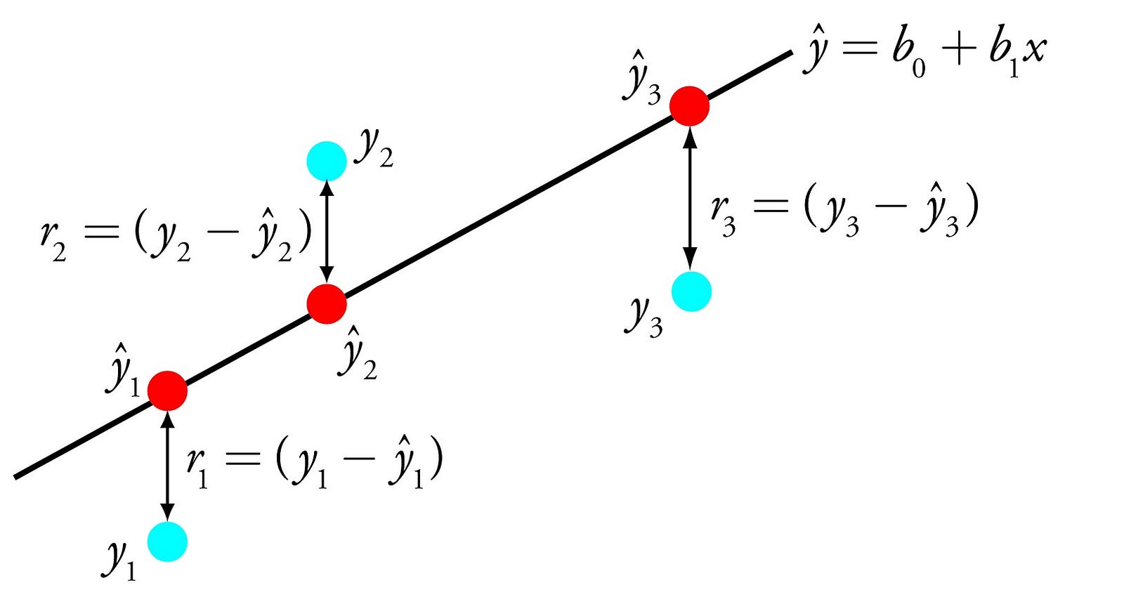
The
representation of linear regression is an equation that describes a
line that best fits the relationship between the input variables (x) and
the output variables (y), by finding specific weightings for the input
variables called coefficients (B).
Linear Regression
For example: y = B0 + B1 * x
We
will predict y given the input x and the goal of the linear regression
learning algorithm is to find the values for the coefficients B0 and B1.
Different
techniques can be used to learn the linear regression model from data,
such as a linear algebra solution for ordinary least squares and
gradient descent optimization.
Linear
regression has been around for more than 200 years and has been
extensively studied. Some good rules of thumb when using this technique
are to remove variables that are very similar (correlated) and to remove
noise from your data, if possible. It is a fast and simple technique
and good first algorithm to try.
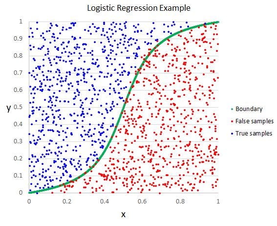
2 — Logistic Regression
Logistic
regression is another technique borrowed by machine learning from the
field of statistics. It is the go-to method for binary classification
problems (problems with two class values).
Logistic
regression is like linear regression in that the goal is to find the
values for the coefficients that weight each input variable. Unlike
linear regression, the prediction for the output is transformed using a
non-linear function called the logistic function.
The
logistic function looks like a big S and will transform any value into
the range 0 to 1. This is useful because we can apply a rule to the
output of the logistic function to snap values to 0 and 1 (e.g. IF less
than 0.5 then output 1) and predict a class value.
Logistic Regression
Because
of the way that the model is learned, the predictions made by logistic
regression can also be used as the probability of a given data instance
belonging to class 0 or class 1. This can be useful for problems where
you need to give more rationale for a prediction.
Like
linear regression, logistic regression does work better when you remove
attributes that are unrelated to the output variable as well as
attributes that are very similar (correlated) to each other. It’s a fast
model to learn and effective on binary classification problems.
3 — Linear Discriminant Analysis
Logistic
Regression is a classification algorithm traditionally limited to only
two-class classification problems. If you have more than two classes
then the Linear Discriminant Analysis algorithm is the preferred linear
classification technique.
The
representation of LDA is pretty straight forward. It consists of
statistical properties of your data, calculated for each class. For a
single input variable this includes:
The mean value for each class.
The variance calculated across all classes.
Linear Discriminant Analysis
Predictions
are made by calculating a discriminate value for each class and making a
prediction for the class with the largest value. The technique assumes
that the data has a Gaussian distribution (bell curve), so it is a good
idea to remove outliers from your data before hand. It’s a simple and
powerful method for classification predictive modeling problems.
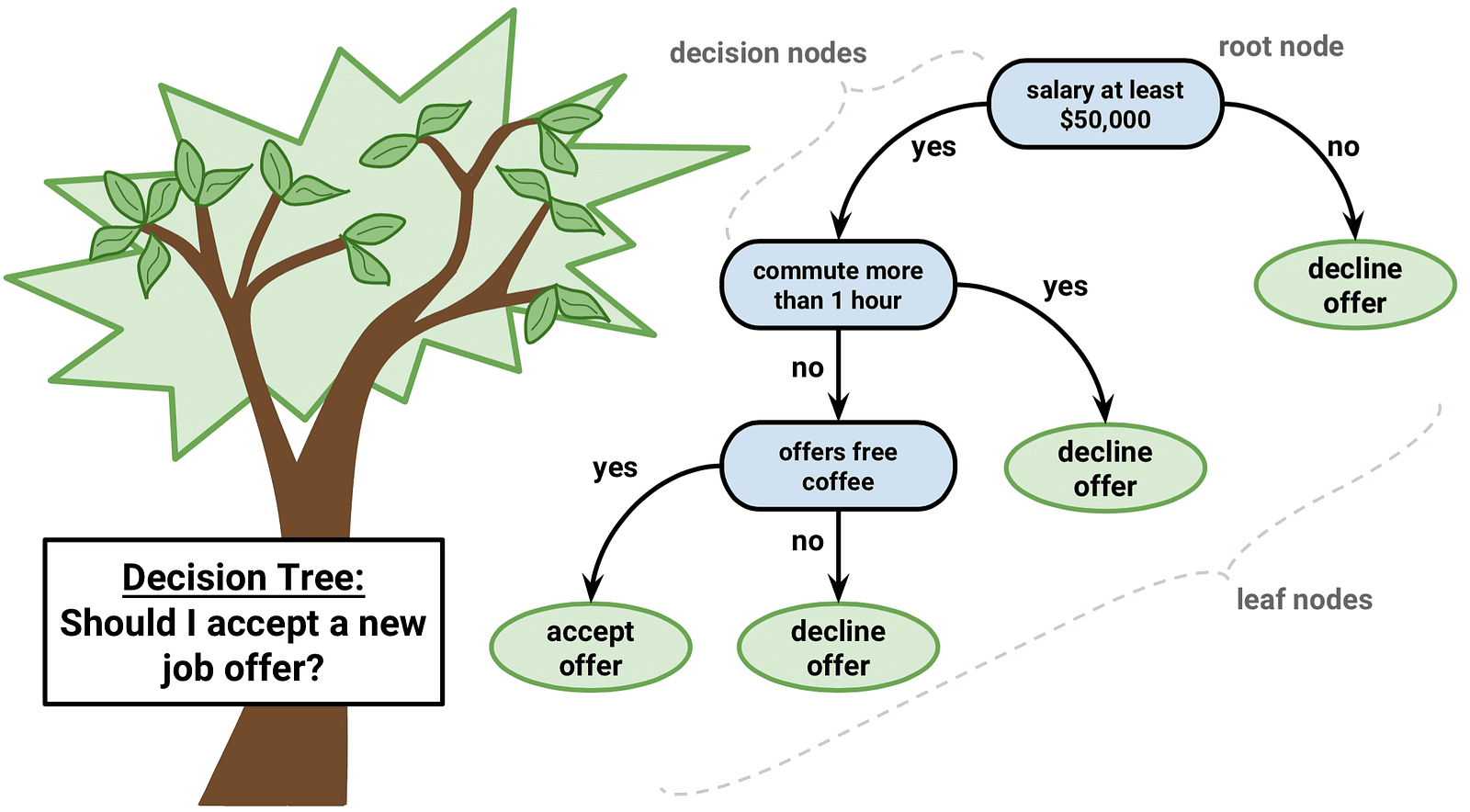
4 — Classification and Regression Trees
Decision Trees are an important type of algorithm for predictive modeling machinelearning.
The
representation of the decision tree model is a binary tree. This is
your binary tree from algorithms and data structures, nothing too fancy.
Each node represents a single input variable (x) and a split point on
that variable (assuming the variable is numeric).
Decision Tree
The
leaf nodes of the tree contain an output variable (y) which is used to
make a prediction. Predictions are made by walking the splits of the
tree until arriving at a leaf node and output the class value at that
leaf node.
Trees
are fast to learn and very fast for making predictions. They are also
often accurate for a broad range of problems and do not require any
special preparation for your data.
5 — Naive Bayes
Naive Bayes is a simple but surprisingly powerful algorithm for predictive modeling.
The
model is comprised of two types of probabilities that can be calculated
directly from your training data: 1) The probability of each class; and
2) The conditional probability for each class given each x value. Once
calculated, the probability model can be used to make predictions for
new data using Bayes Theorem. When your data is real-valued it is common
to assume a Gaussian distribution (bell curve) so that you can easily
estimate these probabilities.
Bayes Theorem
Naive
Bayes is called naive because it assumes that each input variable is
independent. This is a strong assumption and unrealistic for real data,
nevertheless, the technique is very effective on a large range of
complex problems.
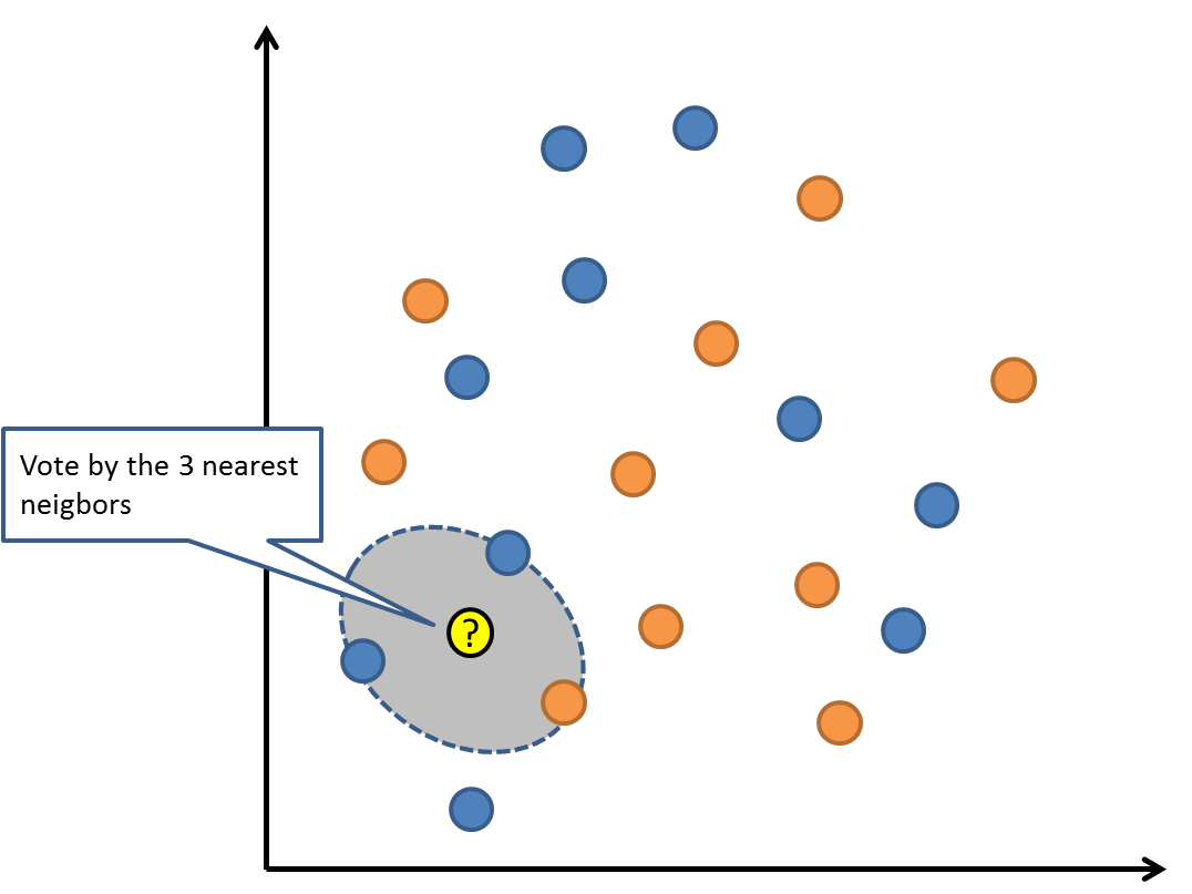
6 — K-Nearest Neighbors
The
KNN algorithm is very simple and very effective. The model
representation for KNN is the entire training dataset. Simple right?
Predictions
are made for a new data point by searching through the entire training
set for the K most similar instances (the neighbors) and summarizing the
output variable for those K instances. For regression problems, this
might be the mean output variable, for classification problems this
might be the mode (or most common) class value.
The
trick is in how to determine the similarity between the data instances.
The simplest technique if your attributes are all of the same scale
(all in inches for example) is to use the Euclidean distance, a number
you can calculate directly based on the differences between each input
variable.
K-Nearest Neighbors
KNN
can require a lot of memory or space to store all of the data, but only
performs a calculation (or learn) when a prediction is needed, just in
time. You can also update and curate your training instances over time
to keep predictions accurate.
The
idea of distance or closeness can break down in very high dimensions
(lots of input variables) which can negatively affect the performance of
the algorithm on your problem. This is called the curse of
dimensionality. It suggests you only use those input variables that are
most relevant to predicting the output variable.
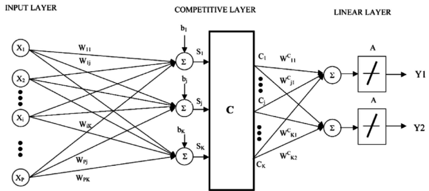
7 — Learning Vector Quantization
A
downside of K-Nearest Neighbors is that you need to hang on to your
entire training dataset. The Learning Vector Quantization algorithm (or
LVQ for short) is an artificial neural network algorithm that allows you
to choose how many training instances to hang onto and learns exactly
what those instances should look like.
Learning Vector Quantization
The
representation for LVQ is a collection of codebook vectors. These are
selected randomly in the beginning and adapted to best summarize the
training dataset over a number of iterations of the learning algorithm.
After learned, the codebook vectors can be used to make predictions just
like K-Nearest Neighbors. The most similar neighbor (best matching
codebook vector) is found by calculating the distance between each
codebook vector and the new data instance. The class value or (real
value in the case of regression) for the best matching unit is then
returned as the prediction. Best results are achieved if you rescale
your data to have the same range, such as between 0 and 1.
If
you discover that KNN gives good results on your dataset try using LVQ
to reduce the memory requirements of storing the entire training
dataset.
8 — Support Vector Machines
Support Vector Machines are perhaps one of the most popular and talked about machine learning algorithms.
A
hyperplane is a line that splits the input variable space. In SVM, a
hyperplane is selected to best separate the points in the input variable
space by their class, either class 0 or class 1. In two-dimensions, you
can visualize this as a line and let’s assume that all of our input
points can be completely separated by this line. The SVM learning
algorithm finds the coefficients that results in the best separation of
the classes by the hyperplane.
Support Vector Machine
The
distance between the hyperplane and the closest data points is referred
to as the margin. The best or optimal hyperplane that can separate the
two classes is the line that has the largest margin. Only these points
are relevant in defining the hyperplane and in the construction of the
classifier. These points are called the support vectors. They support or
define the hyperplane. In practice, an optimization algorithm is used
to find the values for the coefficients that maximizes the margin.
SVM might be one of the most powerful out-of-the-box classifiers and worth trying on your dataset.
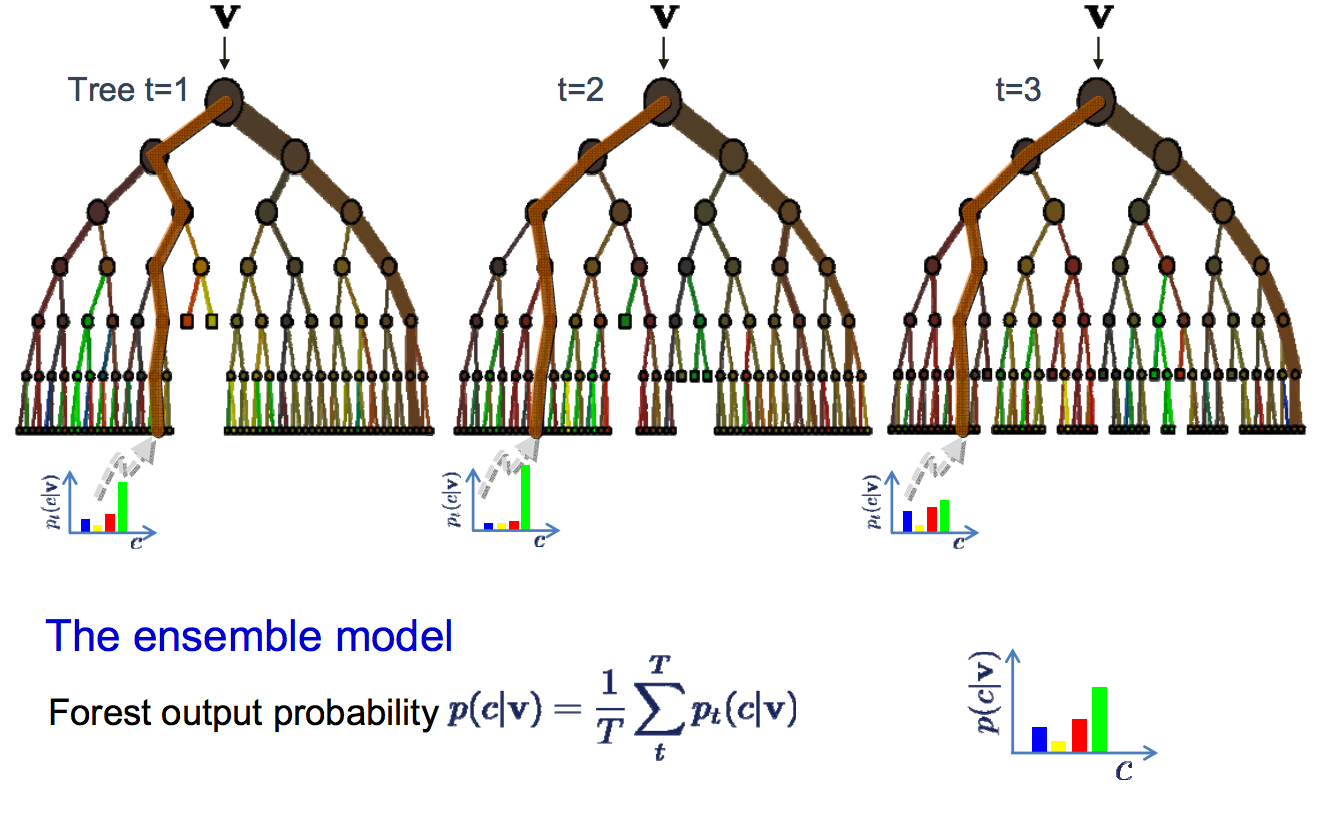
9 — Bagging and Random Forest
Random
Forest is one of the most popular and most powerful machine learning
algorithms. It is a type of ensemble machine learning algorithm called
Bootstrap Aggregation or bagging.
The
bootstrap is a powerful statistical method for estimating a quantity
from a data sample. Such as a mean. You take lots of samples of your
data, calculate the mean, then average all of your mean values to give
you a better estimation of the true mean value.
In
bagging, the same approach is used, but instead for estimating entire
statistical models, most commonly decision trees. Multiple samples of
your training data are taken then models are constructed for each data
sample. When you need to make a prediction for new data, each model
makes a prediction and the predictions are averaged to give a better
estimate of the true output value.
Random Forest
Random
forest is a tweak on this approach where decision trees are created so
that rather than selecting optimal split points, suboptimal splits are
made by introducing randomness.
The
models created for each sample of the data are therefore more different
than they otherwise would be, but still accurate in their unique and
different ways. Combining their predictions results in a better estimate
of the true underlying output value.
If
you get good results with an algorithm with high variance (like
decision trees), you can often get better results by bagging that
algorithm.
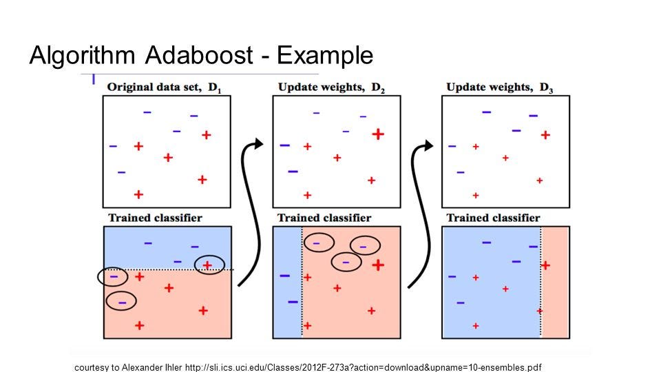
10 — Boosting and AdaBoost
Boosting
is an ensemble technique that attempts to create a strong classifier
from a number of weak classifiers. This is done by building a model from
the training data, then creating a second model that attempts to
correct the errors from the first model. Models are added until the
training set is predicted perfectly or a maximum number of models are
added.
AdaBoost
was the first really successful boosting algorithm developed for binary
classification. It is the best starting point for understanding
boosting. Modern boosting methods build on AdaBoost, most notably
stochastic gradient boosting machines.
AdaBoost
AdaBoost
is used with short decision trees. After the first tree is created, the
performance of the tree on each training instance is used to weight how
much attention the next tree that is created should pay attention to
each training instance. Training data that is hard to predict is given
more weight, whereas easy to predict instances are given less weight.
Models are created sequentially one after the other, each updating the
weights on the training instances that affect the learning performed by
the next tree in the sequence. After all the trees are built,
predictions are made for new data, and the performance of each tree is
weighted by how accurate it was on training data.
Because
so much attention is put on correcting mistakes by the algorithm it is
important that you have clean data with outliers removed.
Last Takeaway
A
typical question asked by a beginner, when facing a wide variety of
machine learning algorithms, is “which algorithm should I use?” The
answer to the question varies depending on many factors, including: (1)
The size, quality, and nature of data; (2) The available computational
time; (3) The urgency of the task; and (4) What you want to do with the
data.
Even
an experienced data scientist cannot tell which algorithm will perform
the best before trying different algorithms. Although there are many
other Machine Learning algorithms, these are the most popular ones. If
you’re a newbie to Machine Learning, these would be a good starting
point to learn.
— —
If you enjoyed this piece, I’d love it if you hit the clap button 👏 so others might stumble upon it. You can find my own code onGitHub, and more of my writing and projects athttps://jameskle.com/. You can also follow me on Twitter, email me directly or find me on LinkedIn. Sign up for my newsletter to receive my latest thoughts on data science, machine learning, and artificial intelligence right at your inbox!