http://www.wildml.com/2015/09/implementing-a-neural-network-from-scratch/
Get the code: To follow along, all the code is also available as an iPython notebook on Github.
In this post we will implement a simple 3-layer neural network from
scratch. We won’t derive all the math that’s required, but I will try to
give an intuitive explanation of what we are doing. I will also point
to resources for you read up on the details.
Here I’m assuming that you are familiar with basic Calculus and
Machine Learning concepts, e.g. you know what classification and
regularization is. Ideally you also know a bit about how optimization
techniques like gradient descent work. But even if you’re not familiar
with any of the above this post could still turn out to be interesting
;)
But why implement a Neural Network from scratch at all? Even if you plan on using Neural Network libraries like
PyBrain
in the future, implementing a network from scratch at least once is an
extremely valuable exercise. It helps you gain an understanding of how
neural networks work, and that is essential for designing effective
models.
One thing to note is that the code examples here aren’t terribly
efficient. They are meant to be easy to understand. In an upcoming post I
will explore how to write an efficient Neural Network implementation
using
Theano.
Generating a dataset
Let’s start by generating a dataset we can play with. Fortunately,
scikit-learn has some useful dataset generators, so we don’t need to write the code ourselves. We will go with the
make_moons function.
|
|
# Generate a dataset and plot it
np.random.seed(0)
X, y = sklearn.datasets.make_moons(200, noise=0.20)
plt.scatter(X[:,0], X[:,1], s=40, c=y, cmap=plt.cm.Spectral)
|

The dataset we generated has two classes, plotted as red and blue
points. You can think of the blue dots as male patients and the red dots
as female patients, with the x- and y- axis being medical measurements.
Our goal is to train a Machine Learning classifier that predicts the
correct class (male of female) given the x- and y- coordinates. Note
that the data is not linearly separable, we can’t draw a straight line
that separates the two classes. This means that linear classifiers, such
as Logistic Regression, won’t be able to fit the data unless you
hand-engineer non-linear features (such as polynomials) that work well
for the given dataset.
In fact, that’s one of the major advantages of Neural Networks. You don’t need to worry about
feature engineering. The hidden layer of a neural network will learn features for you.
Logistic Regression
To demonstrate the point let’s train a Logistic Regression
classifier. It’s input will be the x- and y-values and the output the
predicted class (0 or 1). To make our life easy we use the Logistic
Regression class from
scikit-learn.
|
|
# Train the logistic rgeression classifier
clf = sklearn.linear_model.LogisticRegressionCV()
clf.fit(X, y)
# Plot the decision boundary
plot_decision_boundary(lambda x: clf.predict(x))
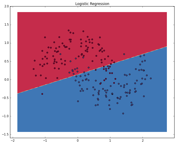
plt.title("Logistic Regression")
|

The graph shows the decision boundary learned by our Logistic
Regression classifier. It separates the data as good as it can using a
straight line, but it’s unable to capture the “moon shape” of our data.
Training a Neural Network
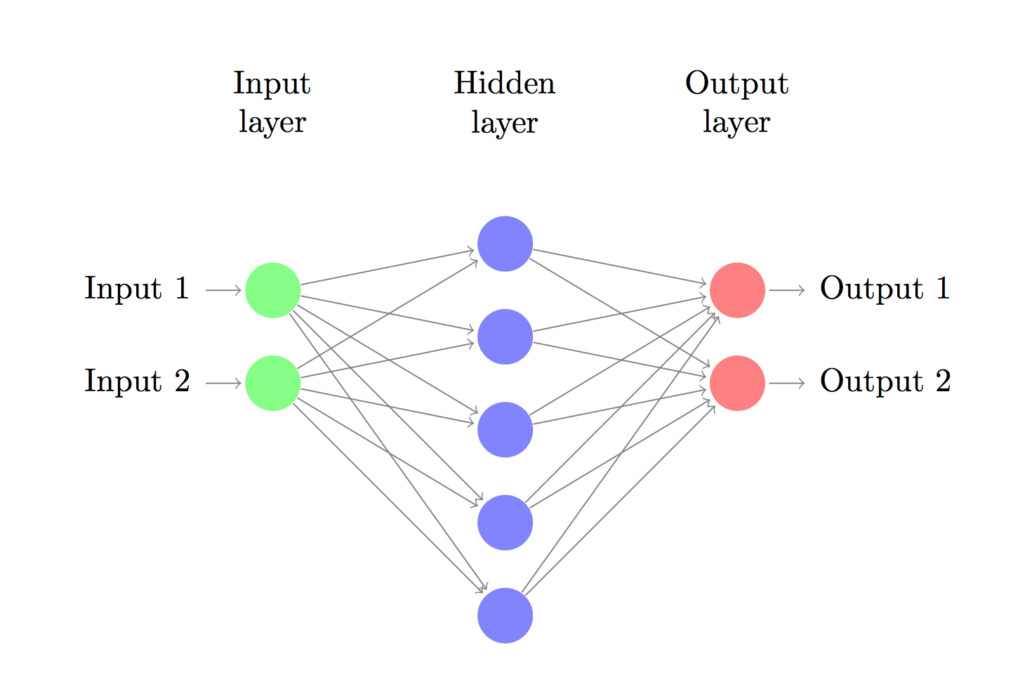
Let’s now build a 3-layer neural network with one input layer, one
hidden layer, and one output layer. The number of nodes in the input
layer is determined by the dimensionality of our data, 2. Similarly, the
number of nodes in the output layer is determined by the number of
classes we have, also 2. (Because we only have 2 classes we could
actually get away with only one output node predicting 0 or 1, but
having 2 makes it easier to extend the network to more classes later
on). The input to the network will be x- and y- coordinates and its
output will be two probabilities, one for class 0 (“female”) and one for
class 1 (“male”). It looks something like this:

We can choose the dimensionality (the number of nodes) of the hidden
layer. The more nodes we put into the hidden layer the more complex
functions we will be able fit. But higher dimensionality comes at a
cost. First, more computation is required to make predictions and learn
the network parameters. A bigger number of parameters also means we
become more prone to overfitting our data.
How to choose the size of the hidden layer? While there are some
general guidelines and recommendations, it always depends on your
specific problem and is more of an art than a science. We will play with
the number of nodes in the hidden later later on and see how it affects
our output.
We also need to pick an
activation function for our hidden
layer. The activation function transforms the inputs of the layer into
its outputs. A nonlinear activation function is what allows us to fit
nonlinear hypotheses. Common chocies for activation functions are
tanh, the
sigmoid function, or
ReLUs. We will use
tanh,
which performs quite well in many scenarios. A nice property of these
functions is that their derivate can be computed using the original
function value. For example, the derivative of

is

. This is useful because it allows us to compute

once and re-use its value later on to get the derivative.
Because we want our network to output probabilities the activation function for the output layer will be the
softmax,
which is simply a way to convert raw scores to probabilities. If you’re
familiar with the logistic function you can think of softmax as its
generalization to multiple classes.
How our network makes predictions
Our network makes predictions using forward propagation, which is
just a bunch of matrix multiplications and the application of the
activation function(s) we defined above. If x is the 2-dimensional input
to our network then we calculate our prediction

(also two-dimensional) as follows:
 \\ z_2 & = a_1W_2 + b_2 \\ a_2 & = \hat{y} = \mathrm{softmax}(z_2) \end{aligned}")

is the input of layer

and

is the output of layer
after applying the activation function.

are parameters of our network, which we need to learn from our training
data. You can think of them as matrices transforming data between
layers of the network. Looking at the matrix multiplications above we
can figure out the dimensionality of these matrices. If we use 500 nodes
for our hidden layer then

,

,

,

. Now you see why we have more parameters if we increase the size of the hidden layer.
Learning the Parameters
Learning the parameters for our network means finding parameters (
)
that minimize the error on our training data. But how do we define the
error? We call the function that measures our error the
loss function. A common choice with the softmax output is the
cross-entropy loss. If we have

training examples and

classes then the loss for our prediction
with respect to the true labels

is given by:
 = - \frac{1}{N} \sum_{n \in N} \sum_{i \in C} y_{n,i} \log\hat{y}_{n,i} \end{aligned}")
The formula looks complicated, but all it really does is sum over our
training examples and add to the loss if we predicted the incorrect
class. So, the further away
(the correct labels) and
(our predictions) are, the greater our loss will be.
Remember that our goal is to find the parameters that minimize our loss function. We can use
gradient descent
to find the minimum. I will implement the most vanilla version of
gradient descent, also called batch gradient descent with a fixed
learning rate. Variations such as SGD (stochastic gradient descent) or
minibatch gradient descent typically perform better in practice. So if
you are serious you’ll want to use one of these, and ideally you would
also
decay the learning rate over time.
As an input, gradient descent needs the gradients (vector of derivatives) of the loss function with respect to our parameters:

,

,

,

. To calculate these gradients we use the famous
backpropagation algorithm,
which is a way to efficiently calculate the gradients starting from the
output. I won’t go into detail how backpropagation works, but there are
many excellent explanations (
here or
here) floating around the web.
Applying the backpropagation formula we find the following (trust me on this):
 \circ \delta_3W_2^T \\ & \frac{\partial{L}}{\partial{W_2}} = a_1^T \delta_3 \\ & \frac{\partial{L}}{\partial{b_2}} = \delta_3\\ & \frac{\partial{L}}{\partial{W_1}} = x^T \delta2\\ & \frac{\partial{L}}{\partial{b_1}} = \delta2 \\ \end{aligned}")
Implementation
Now we are ready for our implementation. We start by defining some useful variables and parameters for gradient descent:
|
|
num_examples = len(X) # training set size
nn_input_dim = 2 # input layer dimensionality
nn_output_dim = 2 # output layer dimensionality
# Gradient descent parameters (I picked these by hand)
epsilon = 0.01 # learning rate for gradient descent
reg_lambda = 0.01 # regularization strength
|
First let’s implement the loss function we defined above. We use this to evaluate how well our model is doing:
1
2
3
4
5
6
7
8
9
10
11
12
13
14
15
|
# Helper function to evaluate the total loss on the dataset
def calculate_loss(model):
W1, b1, W2, b2 = model['W1'], model['b1'], model['W2'], model['b2']
# Forward propagation to calculate our predictions
z1 = X.dot(W1) + b1
a1 = np.tanh(z1)
z2 = a1.dot(W2) + b2
exp_scores = np.exp(z2)
probs = exp_scores / np.sum(exp_scores, axis=1, keepdims=True)
# Calculating the loss
corect_logprobs = -np.log(probs[range(num_examples), y])
data_loss = np.sum(corect_logprobs)
# Add regulatization term to loss (optional)
data_loss += reg_lambda/2 * (np.sum(np.square(W1)) + np.sum(np.square(W2)))
return 1./num_examples * data_loss
|
We also implement a helper function to calculate the output of the
network. It does forward propagation as defined above and returns the
class with the highest probability.
|
|
# Helper function to predict an output (0 or 1)
def predict(model, x):
W1, b1, W2, b2 = model['W1'], model['b1'], model['W2'], model['b2']
# Forward propagation
z1 = x.dot(W1) + b1
a1 = np.tanh(z1)
z2 = a1.dot(W2) + b2
exp_scores = np.exp(z2)
probs = exp_scores / np.sum(exp_scores, axis=1, keepdims=True)
return np.argmax(probs, axis=1)
|
Finally, here comes the function to train our Neural Network. It
implements batch gradient descent using the backpropagation derivates we
found above.
1
2
3
4
5
6
7
8
9
10
11
12
13
14
15
16
17
18
19
20
21
22
23
24
25
26
27
28
29
30
31
32
33
34
35
36
37
38
39
40
41
42
43
44
45
46
47
48
49
50
51
52
53
54
|
# This function learns parameters for the neural network and returns the model.
# - nn_hdim: Number of nodes in the hidden layer
# - num_passes: Number of passes through the training data for gradient descent
# - print_loss: If True, print the loss every 1000 iterations
def build_model(nn_hdim, num_passes=20000, print_loss=False):
# Initialize the parameters to random values. We need to learn these.
np.random.seed(0)
W1 = np.random.randn(nn_input_dim, nn_hdim) / np.sqrt(nn_input_dim)
b1 = np.zeros((1, nn_hdim))
W2 = np.random.randn(nn_hdim, nn_output_dim) / np.sqrt(nn_hdim)
b2 = np.zeros((1, nn_output_dim))
# This is what we return at the end
model = {}
# Gradient descent. For each batch...
for i in xrange(0, num_passes):
# Forward propagation
z1 = X.dot(W1) + b1
a1 = np.tanh(z1)
z2 = a1.dot(W2) + b2
exp_scores = np.exp(z2)
probs = exp_scores / np.sum(exp_scores, axis=1, keepdims=True)
# Backpropagation
delta3 = probs
delta3[range(num_examples), y] -= 1
dW2 = (a1.T).dot(delta3)
db2 = np.sum(delta3, axis=0, keepdims=True)
delta2 = delta3.dot(W2.T) * (1 - np.power(a1, 2))
dW1 = np.dot(X.T, delta2)
db1 = np.sum(delta2, axis=0)
# Add regularization terms (b1 and b2 don't have regularization terms)
dW2 += reg_lambda * W2
dW1 += reg_lambda * W1
# Gradient descent parameter update
W1 += -epsilon * dW1
b1 += -epsilon * db1
W2 += -epsilon * dW2
b2 += -epsilon * db2
# Assign new parameters to the model
model = { 'W1': W1, 'b1': b1, 'W2': W2, 'b2': b2}
# Optionally print the loss.
# This is expensive because it uses the whole dataset, so we don't want to do it too often.
if print_loss and i % 1000 == 0:
print "Loss after iteration %i: %f" %(i, calculate_loss(model))
return model
|
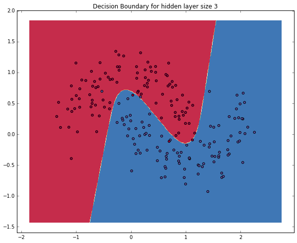
A network with a hidden layer of size 3
Let’s see what happens if we train a network with a hidden layer size of 3.
|
|
# Build a model with a 3-dimensional hidden layer
model = build_model(3, print_loss=True)
# Plot the decision boundary
plot_decision_boundary(lambda x: predict(model, x))
plt.title("Decision Boundary for hidden layer size 3")
|

Yay! This looks pretty good. Our neural networks was able to find a decision boundary that successfully separates the classes.
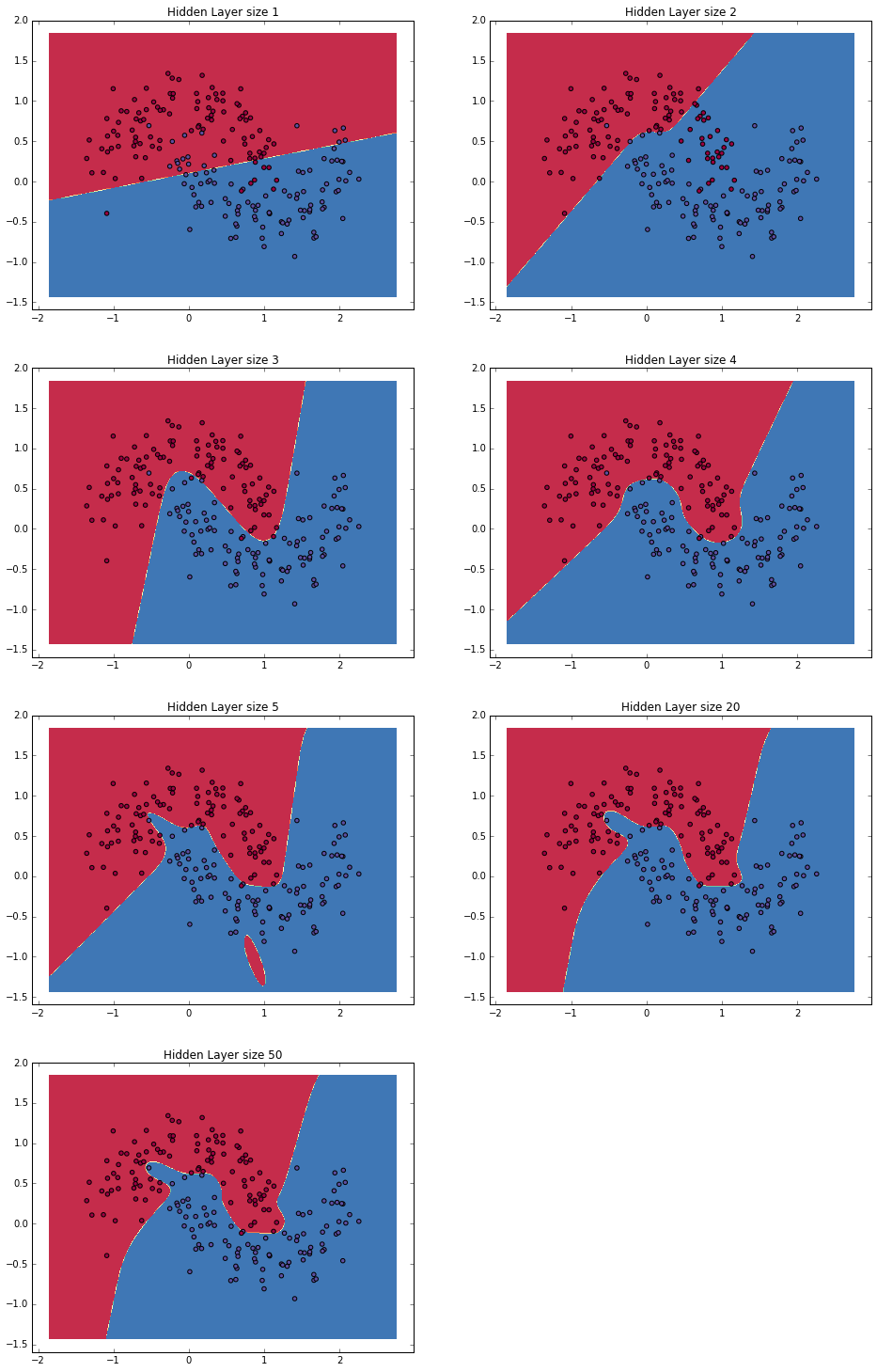
Varying the hidden layer size
In the example above we picked a hidden layer size of 3. Let’s now
get a sense of how varying the hidden layer size affects the result.
|
|
plt.figure(figsize=(16, 32))
hidden_layer_dimensions = [1, 2, 3, 4, 5, 20, 50]
for i, nn_hdim in enumerate(hidden_layer_dimensions):
plt.subplot(5, 2, i+1)
plt.title('Hidden Layer size %d' % nn_hdim)
model = build_model(nn_hdim)
plot_decision_boundary(lambda x: predict(model, x))
plt.show()
|

We can see that a hidden layer of low dimensionality nicely captures
the general trend of our data. Higher dimensionalities are prone to
overfitting. They are “memorizing” the data as opposed to fitting the
general shape. If we were to evaluate our model on a separate test set
(and you should!) the model with a smaller hidden layer size would
likely perform better due to better generalization. We could counteract
overfitting with stronger regularization, but picking the a correct size
for hidden layer is a much more “economical” solution.
Exercises
Here are some things you can try to become more familiar with the code:
- Instead of batch gradient descent, use minibatch gradient descent (more info) to train the network. Minibatch gradient descent typically performs better in practice.
- We used a fixed learning rate
 for gradient descent. Implement an annealing schedule for the gradient descent learning rate (more info).
- We used a
 activation function for our hidden layer. Experiment with other
activation functions (some are mentioned above). Note that changing the
activation function also means changing the backpropagation derivative.
activation function for our hidden layer. Experiment with other
activation functions (some are mentioned above). Note that changing the
activation function also means changing the backpropagation derivative.
- Extend the network from two to three classes. You will need to generate an appropriate dataset for this.
- Extend the network to four layers. Experiment with the layer size.
Adding another hidden layer means you will need to adjust both the
forward propagation as well as the backpropagation code.