Pink
singlet, dyed red hair, plated grey beard, no shoes, John Lennon
glasses. What a character. Imagine the stories he’d have. He parked his
moped and walked into the cafe.
This
cafe is a local favourite. But the chairs aren’t very comfortable. So
I’ll keep this short (spoiler: by short, I mean short compared to the
amount of time you’ll actually spend doing EDA).
When I first started as a Machine Learning Engineer at Max Kelsen, I’d never heard of EDA. There are a bunch of acronyms I’ve never heard of.
I later learned EDA stands for exploratory data analysis.
It’s what you do when you first encounter a data set. But it’s not a once off process. It’s a continual process.
The
past few weeks I’ve been working on a machine learning project.
Everything was going well. I had a model trained on a small amount of
the data. The results were pretty good.
It was time to step it up and add more data. So I did. Then it broke.
I filled up the memory on the cloud computer I was working on. I tried again. Same issue.
There was a memory leak somewhere. I missed something. What changed?
More data.
Maybe
the next sample of data I pulled in had something different to the
first. It did. There was an outlier. One sample which had 68 times the
amount of purchases as the mean (100).
Back
to my code. It wasn’t robust to outliers. It took the outliers value
and applied to the rest of the samples and padded them with zeros.
Instead of having 10 million samples with a length of 100, they all had a length of 6800. And most of that data was zeroes.
I changed the code. Reran the model and training began. The memory leak was patched.
Pause.
The guy with the pink singlet came over. He tells me his name is Johnny.
He continues.
‘The girls got up me for not saying hello.’
‘You can’t win,’ I said.
‘Too right,’ he said.
We
laughed. The girls here are really nice. The regulars get teased.
Johnny is a regular. He told me he has his own farm at home. And his
toenails were painted pink and yellow, alternating, pink, yellow, pink,
yellow.
Johnny left.
Back to it.
What happened? Why the break in the EDA story?
Apart
from introducing you to the legend of Johnny, I wanted to give an
example of how you can think the road ahead is clear but really, there’s
a detour.
EDA is one big detour. There’s no real structured way to do it. It’s an iterative process.
Why do EDA?
When
I started learning machine learning and data science, much of it (all
of it) was through online courses. I used them to create my own AI Masters Degree. All of them provided excellent curriculum along with excellent datasets.
The datasets were excellent because they were ready to be used with machine learning algorithms right out of the box.
You’d download the data, choose your algorithm, call the .fit()
function, pass it the data and all of a sudden the loss value would
start going down and you’d be left with an accuracy metric. Magic.
This
was how the majority of my learning went. Then I got a job as a machine
learning engineer. I thought, finally, I can apply what I’ve been
learning to real-world problems.
Roadblock.
The client sent us the data. I looked at it. WTF was this?
Words, time stamps, more words, rows with missing data, columns, lots of columns. Where were the numbers?
‘How do I deal with this data?’ I asked Athon.
‘You’ll have to do some feature engineering and encode the categorical variables,’ he said, ‘I’ll Slack you a link.’
I went to my digital mentor. Google. ‘What is feature engineering?’
There it was. The next bridge I had to cross. EDA.
You do exploratory data analysis to learn more about the more before you ever run a machine learning model.
You
create your own mental model of the data so when you run a machine
learning model to make predictions, you’ll be able to recognise whether
they’re BS or not.
Rather
than answer all your questions about EDA, I designed this post to spark
your curiosity. To get you to think about questions you can ask of a
dataset.
Where do you start?
How do you explore a mountain range?
Do you walk straight to the top?
How about along the base and try and find the best path?
It
depends on what you’re trying to achieve. If you want to get to the
top, it’s probably good to start climbing sometime soon. But it’s also
probably good to spend some time looking for the best route.
Exploring data is the same. What questions are you trying to solve? Or better, what assumptions are you trying to prove wrong?
You could spend all day debating these. But best to start with something simple, prove it wrong and add complexity as required.
Example time.
Making your first Kaggle submission
You’ve
been learning data science and machine learning online. You’ve heard of
Kaggle. You’ve read the articles saying how valuable it is to practice
your skills on their problems.
Roadblock.
Despite all the good things you’ve heard about Kaggle. You haven’t made a submission yet.
That was me. Until I put my newly acquired EDA skills to work.
You decide it’s time to enter a competition of your own.
You’re
on the Kaggle website. You go to the ‘Start Here’ section. There’s a
dataset containing information about passengers on the Titanic. You
download it and load up a Jupyter Notebook.
What do you do?
What question are you trying to solve?
‘Can I predict survival rates of passengers on the Titanic, based on data from other passengers?’
This seems like a good guiding light.
An EDA checklist
Every
morning, I consult with my personal assistant on what I have to do for
the day. My personal assistant doesn’t talk much. Because my personal
assistant is a notepad. I write down a checklist.
If a checklist is good enough for pilots to use every flight, it’s good enough for data scientists to use with every dataset.
My
morning lists are non-exhaustive, other things come up during the day
which have to be done. But having it creates a little order in the
chaos. It’s same with the EDA checklist below.
An EDA checklist
1. What question(s) are you trying to solve (or prove wrong)? 2. What kind of data do you have and how do you treat different types? 3. What’s missing from the data and how do you deal with it? 4. Where are the outliers and why should you care about them? 5. How can you add, change or remove features to get more out of your data?
We’ll go through each of these.
Response opportunity: What would you add to the list?
What question(s) are you trying to solve?
I put an (s) in the subtitle. Ignore it. Start with one. Don’t worry, more will come along as you go.
For our Titanic dataset example it’s:
Can we predict survivors on the Titanic based on data from other passengers?
Too
many questions will clutter your thought space. Humans aren’t good at
computing multiple things at once. We’ll leave that to the machines.
Sometimes a model isn’t required to make a prediction.
Before we go further, if you’re reading this on a computer, I encourage you to open this Juypter Notebook and try to connect the dots with topics in this post. If you’re reading on a phone, don’t fear, the notebook isn’t going away. I’ve written this article in a way you shouldn’t need the notebook but if you’re like me, you learn best seeing things in practice.
What kind of data do you have and how to treat different types?
You’ve imported the Titanic training dataset.
Let’s check it out.
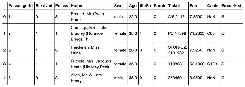
training.head()
.head() shows the top five rows of a dataframe. The rows you’re seeing are from the Kaggle Titanic Training Dataset.
Column
by column, there’s: numbers, numbers, numbers, words, words, numbers,
numbers, numbers, letters and numbers, numbers, letters and numbers and
NaNs, letters. Similar to Johnny’s toenails.
Let’s separate the features out into three boxes, numerical, categorical and not sure.
Columns
of different information are often referred to as features. When you
hear a data scientist talk about different features, they’re probably
talking about different columns in a dataframe.
In the numerical bucket we have, PassengerId, Survived, Pclass, Age, SibSp, Parch and Fare.
The categorical bucket contains Sex and Embarked.
And in not sure we have Name, Ticket and Cabin.
Now we’ve broken the columns down into separate buckets, let’s examine each one.
The Numerical Bucket
Remember our question?
‘Can we predict survivors on the Titanic based on data from other passengers?’
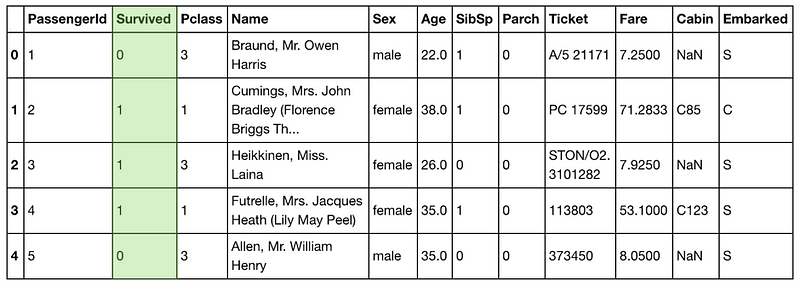
From this, can you figure out which column we’re trying to predict?
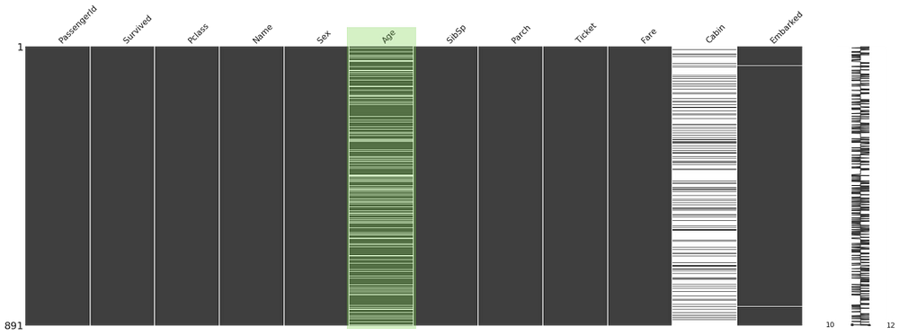
We’re trying to predict the green column using data from the other columns.
The Survivedcolumn.
And because it’s the column we’re trying to predict, we’ll take it out
of the numerical bucket and leave it for the time being.
What’s left?
PassengerId,Pclass, Age, SibSp, Parch and Fare.
Think for a second. If you were trying to predict whether someone survived on the Titanic, do you think their unique PassengerIdwould really help with your cause?
Probably
not. So we’ll leave this column to the side for now too. EDA doesn’t
always have to be done with code, you can use your model of the world to
begin with and use code to see if it’s right later.
How about Pclass, SibSp and Parch?
These are numbers but there’s something different about them. Can you pick it up?
What does Pclass, SibSp and Parch even mean? Maybe we should’ve read the docs more before trying to build a model so quickly.
Google. ‘Kaggle Titanic Dataset’.
Found it.
Pclassis the ticket class, 1 = 1st class, 2 = 2nd class and 3 = 3rd class. SibSp is the number of siblings a passenger has on board. And Parch is the number of parents someone had on board.
This
information was pretty easy to find. But what if you had a dataset
you’d never seen before. What if a real estate agent wanted help
predicting house prices in their city. You check out their data and find
a bunch of columns which you don’t understand.
You email the client.
‘What does Tnummean?’
They respond. ‘Tnum is the number of toilets in a property.’
Good to know.
When
you’re dealing with a new dataset, you won’t always have information
available about it like Kaggle provides. This is where you’ll want to
seek the knowledge of an SME.
Another acronym. Great.
SME stands for subject matter expert.
If you’re working on a project dealing with real estate data, part of
your EDA might involve talking with and asking questions of a real
estate agent. Not only could this save you time, but it could also
influence future questions you ask of the data.
Since no one from the Titanic is alive anymore (RIP (rest in peace) Millvina Dean, the last survivor), we’ll have to become our own SMEs.
There’s something else unique about Pclass, SibSp and Parch. Even though they’re all numbers, they’re also categories.
How so?
Think about it like this. If you can group data together in your head fairly easily, there’s a chance it’s part of a category.
The Pclasscolumn could be labelled, First, Second and Third and it would maintain the same meaning as 1, 2 and 3.
Remember how machine learning algorithms love numbers? Since Pclass, SibSp and Parch are already all in numerical form, we’ll leave them how they are. The same goes for Age.
Phew. That wasn’t too hard.
The Categorical Bucket
In our categorical bucket, we have Sex and Embarked.
These
are categorical variables because you can separate passengers who were
female from those who were male. Or those who embarked on C from those
who embarked from S.
To train a machine learning model, we’ll need a way of converting these to numbers.
How would you do it?
Remember Pclass? 1st = 1, 2nd = 2, 3rd = 3.
How would you do this for Sex and Embarked?
Perhaps you could do something similar for Sex. Female = 1 and male = 2.
As for Embarked, S = 1 and C = 2.
We can change these using the .LabelEncoder() function from the sklearn library.
Wait? Why does C = 0 and S = 2 now? Where’s 1? Hint: There’s an extra category, Q, this takes the number 1. See the data description page on Kaggle for more.
We’ve made some good progress towards turning our categorical data into all numbers but what about the rest of the columns?
Challenge: Now you know Pclass could easily be a categorical variable, how would you turn Age into a categorical variable?
The Not Sure Bucket
Name, Ticket and Cabin are left.
If you were on Titanic, do you think your name would’ve influenced your chance of survival?
It’s unlikely. But what other information could you extract from someone's name?
What if you gave each person a number depending on whether their title was Mr., Mrs. or Miss.?
You could create another column called Title. In this column, those with Mr. = 1, Mrs. = 2 and Miss. = 3.
What you’ve done is created a new feature out of an existing feature. This is called feature engineering.
Converting
titles to numbers is a relatively simple feature to create. And
depending on the data you have, feature engineering can get as
extravagant as you like.
How does this new feature affect the model down the line? This will be something you’ll have to investigate.
For now, we won’t worry about the Name column to make a prediction.
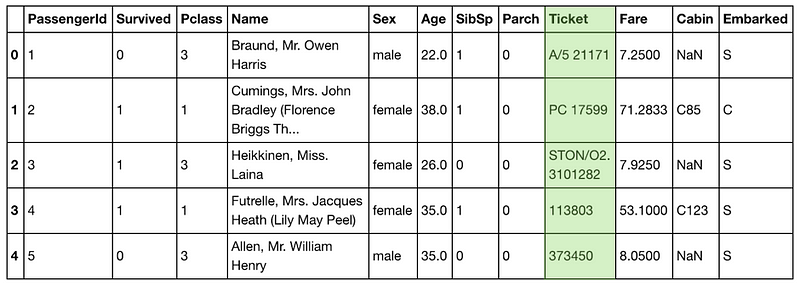
What about Ticket?
The first few examples don’t look very consistent at all. What else is there?
training.Ticket.head(15)
The first 15 entries of the Ticket column.
These
aren’t very consistent either. But think again. Do you think the ticket
number would provide much insight as to whether someone survived?
Maybe
if the ticket number related to what class the person was riding in, it
would have an effect but we already have that information in Pclass.
To save time, we’ll forget the Ticket column for now.
Your
first pass of EDA on a dataset should have the goal of not only raising
more questions about the data but to get a model built using the least
amount of information possible so you’ve got have a baseline to work
from.
Now, what do we do with Cabin?
You know, since I’ve already seen the data, my spidey-senses are telling me it’s a perfect example for the next section.
Challenge: I’ve only listed a couple examples of numerical and categorical data here. Are there any other types of data? How do they differ to these?
What’s missing from the data and how do you deal with it?
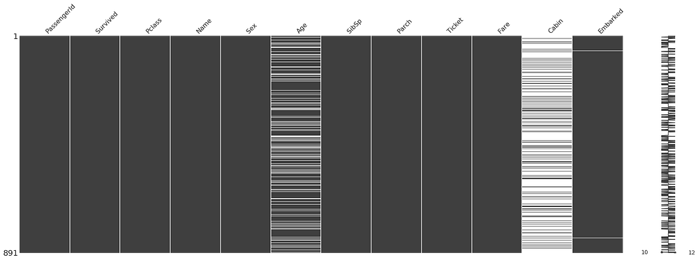
missingno.matrix(train, figsize = (30,10))
The missingno library
is a great quick way to quickly and visually check for holes in your
data, it detects where NaN values (or no values) appear and highlights
them. White lines indicate missing values.
The Cabin column looks like Johnny’s shoes. Not there. There are a fair few missing values in Age too.
How do you predict something when there’s no data?
I don’t know either.
So what are our options when dealing with missing data?
The quickest and easiest way would be to remove every row with missing values. Or remove the Cabin and Age column entirely.
But
there’s a problem here. Machine learning models like more data.
Removing large amounts of data will likely decrease the ability of our
model to predict whether a passenger survived or not.
What’s next?
Imputing values. In other words, filling up the missing data with values calculated from other data.
How would you do this for the Age column?
When we called .head() the Age column had no missing values. But when we look at the whole column, there are plenty of holes.
Could you fill missing values with average age?
There
are drawbacks to this kind of value filling. Imagine you had 1000 total
rows, 500 of which are missing values. You decide to fill the 500
missing rows with the average age of 36.
What happens?
Your
data becomes heavily stacked with the age of 36. How would that
influence predictions on people 36-years-old? Or any other age?
Maybe
for every person with a missing age value, you could find other similar
people in the dataset and use their age. But this is time-consuming and
also has drawbacks.
There are far more advanced methods for filling missing data out of scope for this post. It should be noted, there is no perfect way to fill missing values.
If the missing values in the Age column is a leaky drain pipe the Cabin column is a cracked dam. Beyond saving. For your first model, Cabin is a feature you’d leave out.
Challenge: The Embarked column has a couple of missing values. How would you deal with these? Is the amount low enough to remove them?
Where are the outliers and why you should be paying attention to them?
‘Did you check the distribution?’ Athon asked.
‘I did with the first set of data but not the second set…’ It hit me.
There it was. The rest of the data was being shaped to match the outlier.
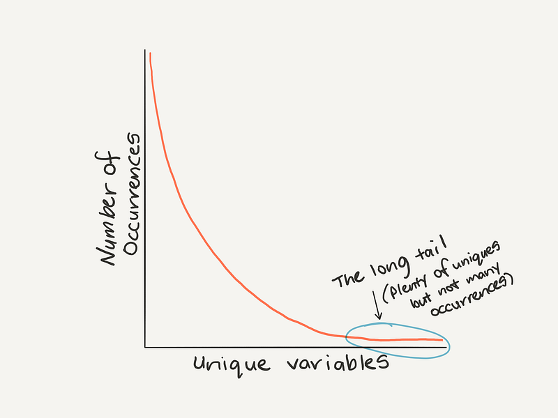
If you look at the number of occurrences of unique values within a dataset, one of the most common patterns you’ll find is Zipf’s law. It looks like this.
Zipf’s
law: The highest occurring variable will have double the number of
occurrences of the second highest occurring variable, triple the amount
of the third and so on.
Remembering
Zipf’s law can help to think about outliers (values towards the end of
the tail don’t occur often and are potential outliers).
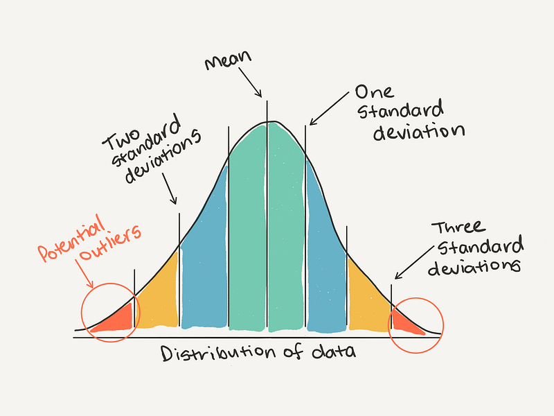
The
definition of an outlier will be different for every dataset. As a
general rule of thumb, you may consider anything more than 3 standard
deviations away from the mean might be considered an outlier.
You could use a general rule to consider anything more than three standard deviations away from the mean as an outlier.
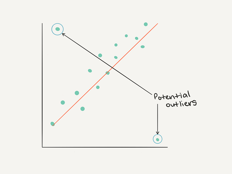
Or from another perspective.
Outliers from the perspective of an (x, y) plot.
How do you find outliers?
Distribution. Distribution. Distribution. Distribution. Four times is enough (I’m trying to remind myself here).
During your first pass of EDA, you should be checking what the distribution of each of your features is.
A
distribution plot will help represent the spread of different values of
data you have across. And more importantly, help to identify potential
outliers.
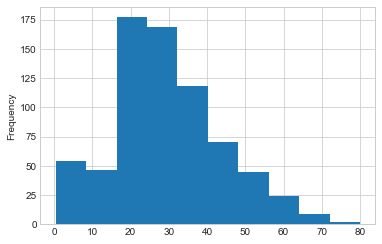
train.Age.plot.hist()
Histogram
plot of the Age column in the training dataset. Are there any outliers
here? Would you remove any age values or keep them all?
Why should you care about outliers?
Keeping
outliers in your dataset may turn out in your model overfitting (being
too accurate). Removing all the outliers may result in your model being
too generalised (it doesn’t do well on anything out of the ordinary). As
always, best to experiment iteratively to find the best way to deal
with outliers.
Challenge: Other than figuring out outliers with the general rule of thumb above, are there any other ways you could identify outliers? If you’re confused about a certain data point, is there someone you could talk to? Hint: the acronym contains the letters M E S.
Getting more out of your data with feature engineering
The Titanic dataset only has 10 features. But what if your dataset has hundreds? Or thousands? Or more? This isn’t uncommon.
During
your exploratory data analysis process, once you’ve started to form an
understanding AND you’ve got an idea of the distributions AND you’ve
found some outliers AND you’ve dealt with them, the next biggest chunk
of your time will be spent on feature engineering.
Feature engineering can be broken down into three categories: adding, removing and changing.
The Titanic dataset started out in pretty good shape. So far, we’ve only had to change a few features to be numerical in nature.
However, data in the wild is different.
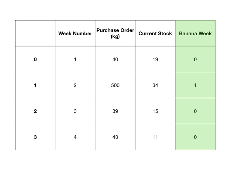
Say
you’re working on a problem trying to predict the changes in banana
stock requirements of a large supermarket chain across the year.
Your
dataset contains a historical record of stock levels and previous
purchase orders. You're able to model these well but you find there are a
few times throughout the year where stock levels change irrationally.
Through your research, you find during a yearly country-wide
celebration, banana week, the stock levels of bananas plummet. This
makes sense. To keep up with the festivities, people buy more bananas.
To
compensate for banana week and help the model learn when it occurs, you
might add a column to your data set with banana week or not banana
week.
# We know Week 2 is a banana week so we can set it using np.where()
A simple example of adding a binary feature to dictate whether a week was banana week or not.
Adding
a feature like this might not be so simple. You could find adding the
feature does nothing at all since the information you’ve added is
already hidden within the data. As in, the purchase orders for the past
few years during banana week are already higher than other weeks.
What about removing features?
We’ve done this as well with the Titanic dataset. We dropped the Cabin column because it was missing so many values before we even ran a model.
But what about if you’ve already run a model using the features left over?
This is where feature contribution comes in. Feature contribution is a way of figuring out how much each feature influences the model.
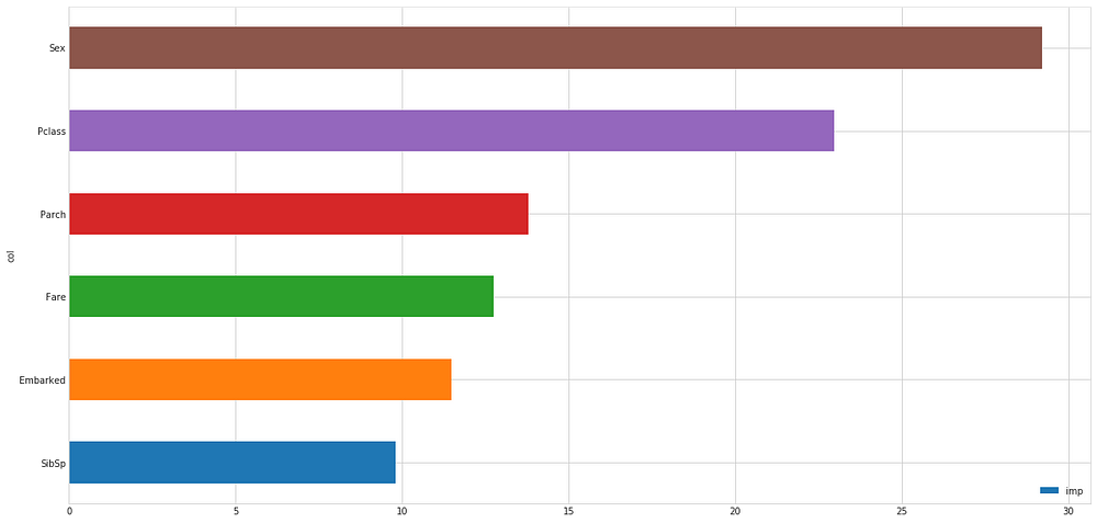
An
example of a feature contribution graph using Sex, Pclass, Parch, Fare,
Embarked and SibSp features to predict who would survive on the
Titanic. If you’ve seen the movie, why does this graph make sense? If
you haven’t, think about it anyway. Hint: ‘Save the women and children!’
Why is this information helpful?
Knowing how much a feature contributes to a model can give you direction as to where to go next with your feature engineering.
In our Titanic example, we can see the contribution of Sex and Pclass were the highest. Why do think this is?
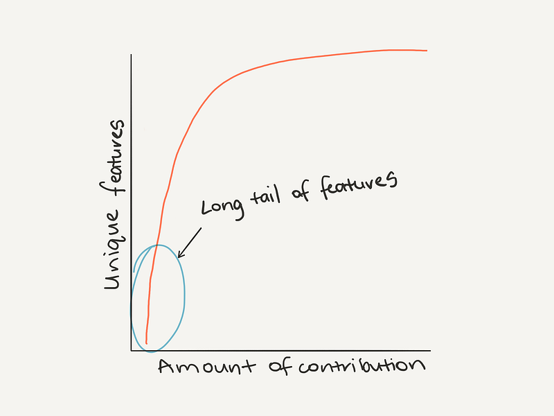
What
if you had more than 10 features? How about 100? You could do the same
thing. Make a graph showing the feature contributions of 100 different
features. ‘Oh, I’ve seen this before!’
Zipf’s law back at it again. The top features have far more to contribute than the bottom features.
Zipf’s law at play with different features and their contribution to a model.
Seeing this, you might decide to cut the lesser contributing features and improve the ones contributing more.
Why would you do this?
Removing
features reduces the dimensionality of your data. It means your model
has fewer connections to make to figure out the best way of fitting the
data.
You might find removing features means your model can get the same (or better) results on fewer data and in less time.
Like Johnny is a regular at the cafe I’m at, feature engineering is a regular part of every data science project.
Challenge: What are other methods of feature engineering? Can you combine two features? What are the benefits of this?
Building your first model(s)
Finally. We’ve been through a bunch of steps to get our data ready to run some models.
If
you’re like me, when you started learning data science, this is the
part you learned first. All the stuff above had already been done by
someone else. All you had to was fit a model on it.
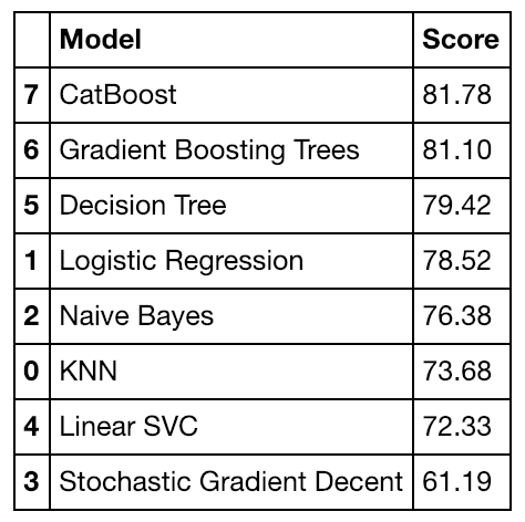
Our Titanic dataset is small. So we can afford to run a multitude of models on it to figure out which is the best to use.
Notice how I put an (s) in the subtitle, you can pay attention to this one.
Cross-validation
accuracy scores from a number of different models I tried using to
predict whether a passenger would survive or not.
But
once you’ve had some practice with different datasets, you’ll start to
figure out what kind of model usually works best. For example, most
recent Kaggle competitions have been won with ensembles (combinations)
of different gradient boosted tree algorithms.
Once you’ve built a few models and figured out which is best, you can start to optimise the best one through hyperparameter tuning.
Think of hyperparameter tuning as adjusting the dials on your oven when
cooking your favourite dish. Out of the box, the preset setting on the
oven works pretty well but out of experience you’ve found lowering the
temperature and increasing the fan speed brings tastier results.
It’s
the same with machine learning algorithms. Many of them work great out
of the box. But with a little tweaking of their parameters, they work
even better.
But no matter what, even the best machine learning algorithm won’t result in a great model without adequate data preparation.
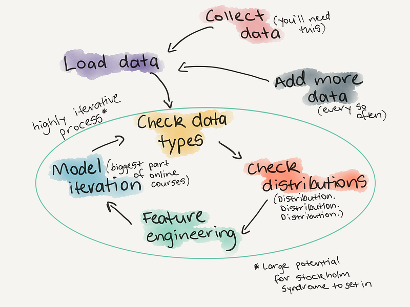
EDA and model building is a repeating circle.
The EDA circle of life.
A final challenge (and some extra-curriculum)
I left the cafe. My ass was sore.
At
the start of this article, I said I’d keep it short. You know how that
turned out. It will be the same as your EDA iterations. When you think
you’re done. There’s more.
We covered a non-exhaustive EDA checklist with the Titanic Kaggle dataset as an example.
1. What question are you trying to solve (or prove wrong)?
Start with the simplest hypothesis possible. Add complexity as needed.
2. What kind of data do you have?
Is your data numerical, categorical or something else? How do you deal with each kind?
3. What’s missing from the data and how do you deal with?
Why
is the data missing? Missing data can be a sign in itself. You’ll never
be able to replace it with anything as good as the original but you can
try.
4. Where are the outliers and why should pay attention to them?
Distribution.
Distribution. Distribution. Three times is enough for the summary.
Where are the outliers in your data? Do you need them or are they
damaging your model?
5. How can you add, change or remove features to get more out of your data?
The
default rule of thumb is more data = good. And following this works
well quite often. But is there anything you can remove get the same
results? Less but better? Start simple.
Data
science isn’t always about getting answers out of data. It’s about
using data to figure out what assumptions of yours were wrong. The most
valuable skill a data scientist can cultivate is a willingness to be
wrong.
There are examples of everything we’ve discussed here (and more) in the notebook on GitHub and a video of me going through the notebook step by step on YouTube (the coding starts at 5:05).
FINAL BOSS CHALLENGE: If you’ve never entered a Kaggle competition before, and want to practice EDA, now’s your chance. Take the notebook I’ve created, rewrite it from top to bottom and improve on my result. If you do, let me know and I’ll share your work on my LinkedIn. Get after it.
Extra-curriculum bonus:Daniel Formoso's notebook is one of the best resources you’ll find for an extensive look at EDA on a Census Income Dataset. After you’ve completed the Titanic EDA, this is a great next step to check out.
If you’ve got something on your mind you think this article is missing, leave a response below or send me a note and I’ll be happy to get back to you.
I took a Deep Learning course through The Bradfield School of Computer Science in June. This series is a journal about what I learned in class, and what I’ve learned since.
This
is the first article in this series, and is is about the recommended
preparation for the Deep Learning course and what we learned in the
first class. Read the second article here, and the third here.
Although
normally the “prework” comes before the introduction, I’m going to give
the 30,000 foot view of the fields of artificial intelligence, machine
learning, and deep learning at the top. I have found that this context
can really help us understand why the prerequisites seem so broad, and
help us study just the essentials. Besides, the history and landscape of
artificial intelligence is interesting, so lets dive in!
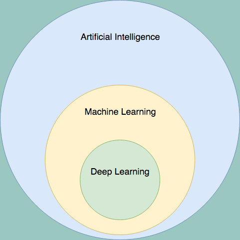
Artificial Intelligence, Machine Learning, and Deep Learning
Deep
learning is a subset of machine learning. Machine learning is a subset
of artificial intelligence. Said another way — all deep learning
algorithms are machine learning algorithms, but many machine learning
algorithms do not use deep learning. As a Venn Diagram, it looks like
this:
Deep learning refers specifically to a class of algorithm called a neural network,
and technically only to “deep” neural networks (more on that in a
second). This first neural network was invented in 1949, but back then
they weren’t very useful. In fact, from the 1970’s to the 2010’s
traditional forms of AI would consistently outperform neural network
based models.
These
non-learning types of AI include rule based algorithms (imagine an
extremely complex series of if/else blocks); heuristic based AIs such as
A* search; constraint satisfaction algorithms like Arc Consistency; tree search algorithms such as minimax (used by the famous Deep Blue chess AI); and more.
There
were two things preventing machine learning, and especially deep
learning, from being successful. Lack of availability of large datasets
and lack of availability of computational power. In 2018 we have
exabytes of data, and anyone with an AWS account and a credit card has
access to a distributed supercomputer. Because of the new availability
of data and computing power, Machine learning — and especially deep
learning — has taken the AI world by storm.
Supervised
learning algorithms work by forcing the machine to repeatedly make
predictions. Specifically, we ask it to make predictions about data that
we (the humans) already know the correct answer for. This is called
“labeled data” — the label is whatever we want the machine to predict.
Here’s
an example: let’s say we wanted to build an algorithm to predict if
someone will default on their mortgage. We would need a bunch of
examples of people who did and did not default on their mortgages. We
will take the relevant data about these people; feed them into the
machine learning algorithm; ask it to make a prediction about each
person; and after it guesses we tell the machine what the right answer
actually was. Based on how right or wrong it was the machine learning
algorithm changes how it makes predictions.
We repeat this process many many
times, and through the miracle of mathematics, our machine’s
predictions get better. The predictions get better relatively slowly
though, which is why we need so much data to train these algorithms.
Machine learning algorithms such as linear regression, support vector machines, and decision trees
all “learn” in different ways, but fundamentally they all apply this
same process: make a prediction, receive a correction, and adjust the
prediction mechanism based on the correction. At a high level, it’s
quite similar to how a human learns.
Recall
that deep learning is a subset of machine learning which focuses on a
specific category of machine learning algorithms called neural networks.
Neural networks were originally inspired by the way human brains
work — individual “neurons” receive “signals” from other neurons and in
turn send “signals” to other “neurons”. Each neuron transforms the
incoming “signals” in some way, and eventually an output signal is
produced. If everything went well that signal represents a correct
prediction!
This
is a helpful mental model, but computers are not biological brains.
They do not have neurons, or synapses, or any of the other biological
mechanisms that make brains work. Because the biological model breaks
down, researchers and scientists instead use graph theory to model
neural networks — instead of describing neural networks as “artificial
brains”, they describe them as complex graphs with powerful properties.
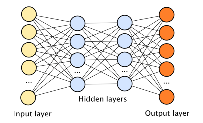
Viewed
through the lens of graph theory a neural network is a series of layers
of connected nodes; each node represents a “neuron” and each connection
represents a “synapse”.
Different kinds of nets have different kinds of connections. The
simplest form of deep learning is a deep neural network. A deep neural
network is a graph with a series of fully connected layers. Every
node in a particular layer has an edge to every node in the next layer;
each of these edges is given a different weight. The whole series of
layers is the “brain”. It turns out, if the weights on all these edges
are set just right these graphs can do some incredible “thinking”.
Ultimately,
the Deep Learning Course will be about how to construct different
versions of these graphs; tune the connection weights until the system
works; and try to make sure our machine does what we think
it’s doing. The mechanics that make Deep Learning work, such as
gradient descent and backpropagation, combine a lot of ideas from
different mathematical disciplines. In order to really understand neural networks we need some math background.
Background Knowledge — A Little Bit Of Everything
Given how easy to use libraries like PyTorch and TensorFlow are, it’s really tempting to say, “you don’t need the math that much.”
But after doing the required reading for the two classes, I’m glad I
have some previous math experience. A subset of topics from linear
algebra, calculus, probability, statistics, and graph theory have
already come up.
Getting
this knowledge at university would entail taking roughly 5 courses.
Calculus 1, 2 and 3; linear algebra; and computer science 101. Luckily,
you don’t need each of those fields in their entirety. Based on what I’ve seen so far, this is what I would recommend studying if you want to get into neural networks yourself:
From linear algebra, you need to know the dot product, matrix multiplication (especially the rules for multiplying matrices with different sizes), and transposes. You
don’t have to be able to do these things quickly by hand, but you
should be comfortable enough to do small examples on a whiteboard or
paper. You should also feel comfortable working with “multidimensional
spaces” — deep learning uses a lot of many dimensional vectors.
I love 3Blue1Brown’s Essence of Linear Algebra
for a refresher or an introduction into linear algebra. Additionally,
compute a few dot products and matrix multiplications by hand (with
small vector/matrix sizes). Although we use graph theory to model neural
networks these graphs are represented in the computer by matrices and
vectors for efficiency reasons. You should be comfortable both thinking
about and programming with vectors and matrices.
From calculus you need to know the derivative, and you ideally should know it pretty well. Neural networks involve simple derivatives, the chain rule, partial derivatives, and the gradient. The derivative is used by neural nets to solve optimization problems,
so you should understand how the derivative can be used to find the
“direction of greatest increase”. A good intuition is probably enough,
but if you solve a couple simple optimization problems using the derivative, you’ll be happy you did. 3Blue1Brown also has an Essence of Calculus series, which is lovely as a more holistic review of calculus.
Gradient
descent and backpropagation both make heavy use of derivatives to fine
tune the networks during training. You don’t have to know how to solve
big complex derivatives with compounding chain and product rules, but
having a feel for partial derivatives with simple equations helps a lot.
From probability and statistics, you should know about common distributions, the idea of metrics, accuracy vs precision,
and hypothesis testing. By far the most common applications of neural
networks are to make predictions or judgements of some kind. Is this a
picture of a dog? Will it rain tomorrow? Should I show Tyler this advertisement, or that one? Statistics and probability will help us assess the accuracy and usefulness of these systems.
It’s
worth noting that the statistics appear more on the applied side; the
graph theory, calculus, and linear algebra all appear on the
implementation side. I think it’s best to understand both, but if you’re
only going to be using a library like TensorFlow and are not interested in implementing these algorithms yourself — it might be wise to focus on the statistics more than the calculus & linear algebra.
Finally,
the graph theory. Honestly, if you can define the terms “vertex”,
“edge” and “edge weight” you’ve probably got enough graph theory under
your belt. Even this “Gentle Introduction” has more information than you need.
In the next article in this series I’ll be examining Deep Neural Networks and how they are constructed. See you then!
To
learn more about my journey to graduate school, and learn what I’m
learning about machine learning, genetics, and bioinformatics you can:
sign up for the Weekly Lab Report, read The Once and Future Student, become a patron on Patreon, or just follow me here on Medium.
PyOD is a comprehensive and scalable Python toolkit for detecting outlying objects in
multivariate data. This exciting yet challenging field is commonly referred as
Outlier Detection
or Anomaly Detection.
Since 2017, PyOD has been successfully used in various academic researches and
commercial products [18][19][20].
PyOD is featured for:
Unified APIs, detailed documentation, and interactive examples across various algorithms.
Advanced models, including Neural Networks/Deep Learning and Outlier Ensembles.
Optimized performance with JIT and parallelization when possible, using numba and joblib.
Compatible with both Python 2 & 3 (scikit-learn compatible as well).
Important Notes:
PyOD contains neural network based models, e.g., AutoEncoders, which are
implemented in Keras. However, PyOD would NOT install Keras and/or
TensorFlow automatically. This reduces the risk of damaging your local copies.
If you want to use neural net based models, you should install Keras and back-end libraries like TensorFlow manually.
An instruction is provided: neural-net FAQ.
Similarly, some models, e.g., XGBOD, depend on xgboost, which would NOT be installed by default. Key Links and Resources: