Weight Initialization in Neural Networks: A Journey From the Basics to Kaiming

https://medium.com/@jamesdell/weight-initialization-in-neural-networks-a-journey-from-the-basics-to-kaiming-954fb9b47c79

I’d like to invite you to join me on an exploration through different approaches to initializing layer weights in neural networks. Step-by-step, through various short experiments and thought exercises, we’ll discover why adequate weight initialization is so important in training deep neural nets. Along the way we’ll cover various approaches that researchers have proposed over the years, and finally drill down on what works best for the contemporary network architectures that you’re most likely to be working with.

The examples to follow come from my own re-implementation of a set of notebooks that Jeremy Howard covered in the latest version of fast.ai’s Deep Learning Part II course, currently being held this spring, 2019, at USF’s Data Institute.

Why Initialize Weights

The aim of weight initialization is to prevent layer activation outputs from exploding or vanishing during the course of a forward pass through a deep neural network. If either occurs, loss gradients will either be too large or too small to flow backwards beneficially, and the network will take longer to converge, if it is even able to do so at all.

Matrix multiplication is the essential math operation of a neural network. In deep neural nets with several layers, one forward pass simply entails performing consecutive matrix multiplications at each layer, between that layer’s inputs and weight matrix. The product of this multiplication at one layer becomes the inputs of the subsequent layer, and so on and so forth.

For a quick-and-dirty example that illustrates this, let’s pretend that we have a vector x that contains some network inputs. It’s standard practice when training neural networks to ensure that our inputs’ values are scaled such that they fall inside such a normal distribution with a mean of 0 and a standard deviation of 1.

Let’s also pretend that we have a simple 100-layer network with no activations , and that each layer has a matrix a that contains the layer’s weights. In order to complete a single forward pass we’ll have to perform a matrix multiplication between layer inputs and weights at each of the hundred layers, which will make for a grand total of 100 consecutive matrix multiplications.

It turns out that initializing the values of layer weights from the same standard normal distribution to which we scaled our inputs is never a good idea. To see why, we can simulate a forward pass through our hypothetical network.

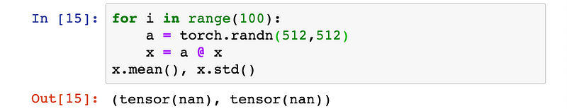
Whoa! Somewhere during those 100 multiplications, the layer outputs got so big that even the computer wasn’t able to recognize their standard deviation and mean as numbers. We can actually see exactly how long that took to happen.

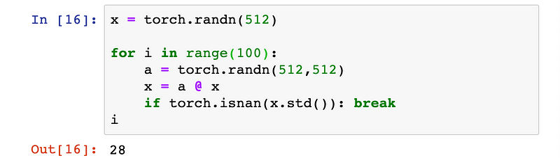
The activation outputs exploded within 29 of our network’s layers. We clearly initialized our weights to be too large.

Unfortunately, we also have to worry about preventing layer outputs from vanishing. To see what happens when we initialize network weights to be too small — we’ll scale our weight values such that, while they still fall inside a normal distribution with a mean of 0, they have a standard deviation of 0.01.

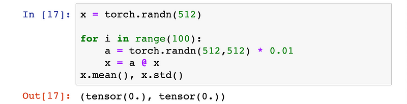
During the course of the above hypothetical forward pass, the activation outputs completely vanished.

To sum it up, if weights are initialized too large, the network won’t learn well. The same happens when weights are initialized too small.

How can we find the sweet spot?

Remember that as mentioned above, the math required to complete a forward pass through a neural network entails nothing more than a succession of matrix multiplications. If we have an output y that is the product of a matrix multiplication between our input vector x and weight matrix a, each element i in y is defined as

where i is a given row-index of weight matrix a, k is both a given column-index in weight matrix a and element-index in input vector x, and n is the range or total number of elements in x. This can also be defined in Python as:

y[i] = sum([c*d for c,d in zip(a[i], x)])

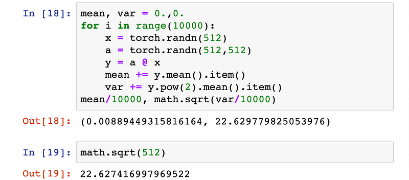
We can demonstrate that at a given layer, the matrix product of our inputs x and weight matrix a that we initialized from a standard normal distribution will, on average, have a standard deviation very close to the square root of the number of input connections, which in our example is √512.

This property isn’t surprising if we view it in terms of how matrix multiplication is defined: in order to calculate y we sum 512 products of the element-wise multiplication of one element of the inputs x by one column of the weights a. In our example where both x and a are initialized using standard normal distributions, each of these 512 products would have a mean of 0 and standard deviation of 1.

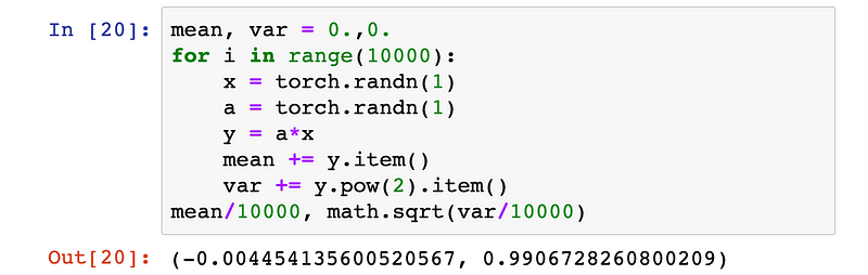
It then follows that the sum of these 512 products would have a mean of 0, variance of 512, and therefore a standard deviation of √512.

And this is why in our example above we saw our layer outputs exploding after 29 consecutive matrix multiplications. In the case of our bare-bones 100-layer network architecture, what we’d like is for each layer’s outputs to have a standard deviation of about 1. This conceivably would allow us to repeat matrix multiplications across as many network layers as we want, without activations exploding or vanishing.

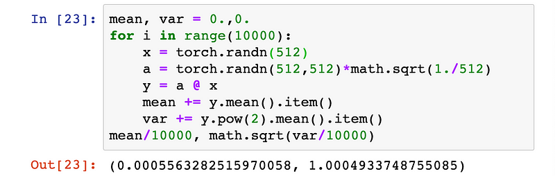
If we first scale the weight matrix a by dividing all its randomly chosen values by √512, the element-wise multiplication that fills in one element of the outputs y would now, on average, have a variance of only 1/√512.

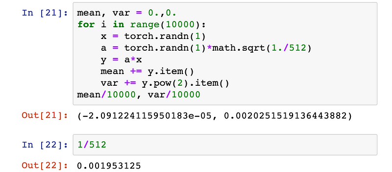
This means that the standard deviation of the matrix y, which contains each of the 512 values that are generated by way of the matrix multiplication between inputs x and weights a, would be 1. Let’s confirm this experimentally.

Now let’s re-run our quick-and-dirty 100-layer network. As before, we first choose layer weights at random from standard normal distribution inside [-1,1], but this time we scale those weights by 1/√n, where n is the number of network input connections at a layer, which is 512 in our example.

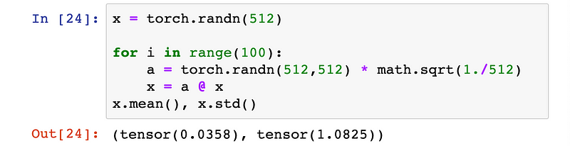
Success! Our layer outputs neither exploded nor vanished, even after 100 of our hypothetical layers.

While at first glance it may seem like at this point we can call it a day, real-world neural networks aren’t quite as simple as our first example may seem to indicate. For the sake of simplicity, activation functions were omitted. However, we’d never do this in real life. It’s thanks to the placement of these non-linear activation functions at the tail end of network layers, that deep neural nets are able create close approximations of intricate functions that describe real-world phenomena, which can then be used to generate astoundingly impressive predictions, such as the classification of handwriting samples.

Xavier Initialization

Up until a few years ago, most commonly used activation functions were symmetric about a given value, and had ranges that asymptotically approached values that were plus/minus a certain distance from this midpoint. The hyperbolic tangent and softsign functions exemplify this class of activations.

Tanh and softsign activation functions. Credit: Sefik Ilkin Serengil’s blog.

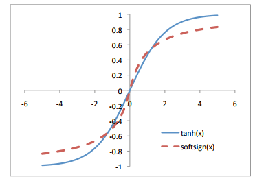
We’ll add a hyperbolic tangent activation function after each layer our hypothetical 100-layer network, and then see what happens when we use our home-grown weight initialization scheme where layer weights are scaled by 1/√n.

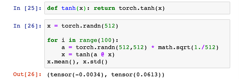
The standard deviation of activation outputs of the 100th layer is down to about 0.06. This is definitely on the small side, but at least activations haven’t totally vanished!

As intuitive as the journey to discovering our home-grown weight init strategy may now seem in retrospect, you may be surprised to hear that as recently as 2010, this was not the conventional approach for initializing weight layers.

When Xavier Glorot and Yoshua Bengio published their landmark paper titled Understanding the difficulty of training deep feedforward neural networks, the “commonly used heuristic” to which they compared their experiments was that of initializing weights from a uniform distribution in [-1,1] and then scaling by 1/√n.

It turns out this “standard” approach doesn’t actually work that well.

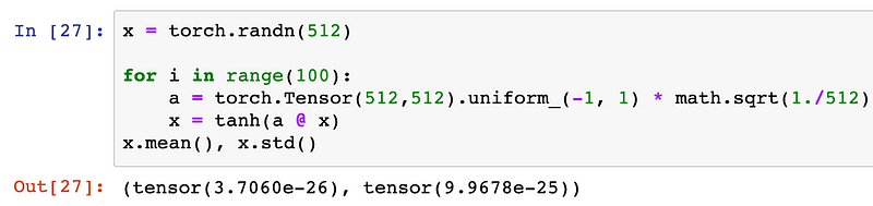
Re-running our 100-layer tanh network with “standard” weight initialization caused activation gradients to become infinitesimally small — they’re just about as good as vanished.

This poor performance is actually what spurred Glorot and Bengio to propose their own weight initialization strategy, which they referred to as “normalized initialization” in their paper, and which is now popularly termed “Xavier initialization.”

Xavier initialization sets a layer’s weights to values chosen from a random uniform distribution that’s bounded between

where nᵢ is the number of incoming network connections, or “fan-in,” to the layer, and nᵢ₊₁ is the number of outgoing network connections from that layer, also known as the “fan-out.”

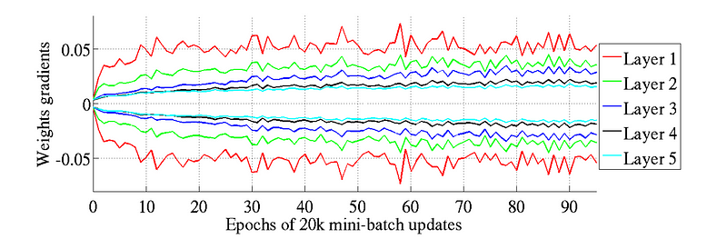
Glorot and Bengio believed that Xavier weight initialization would maintain the variance of activations and back-propagated gradients all the way up or down the layers of a network. In their experiments they observed that Xavier initialization enabled a 5-layer network to maintain near identical variances of its weight gradients across layers.

With Xavier init. Credit: Glorot & Bengio.

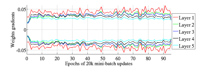
Conversely, it turned out that using “standard” initialization brought about a much bigger gap in variance between weight gradients at the network’s lower layers, which were higher, and those at its top-most layers, which were approaching zero.

Without Xavier init. Credit: Glorot & Bengio.

To drive the point home, Glorot and Bengio demonstrated that networks initialized with Xavier achieved substantially quicker convergence and higher accuracy on the CIFAR-10 image classification task.

Let’s re-run our 100-layer tanh network once more, this time using Xavier initialization:

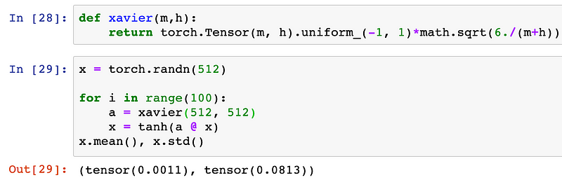
In our experimental network, Xavier initialization performs pretty identical to the home-grown method that we derived earlier, where we sampled values from a random normal distribution and scaled by the square root of number of incoming network connections, n.

Kaiming Initialization

Conceptually, it makes sense that when using activation functions that are symmetric about zero and have outputs inside [-1,1], such as softsign and tanh, we’d want the activation outputs of each layer to have a mean of 0 and a standard deviation around 1, on average. This is precisely what our home-grown method and Xavier both enable.

But what if we’re using ReLU activation functions? Would it still make sense to want to scale random initial weight values in the same way?

ReLU activation function. Credit: Kanchan Sarkar’s blog.

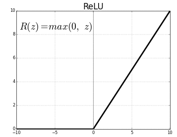
To see what would happen, let’s use a ReLU activation instead of tanh in one of our hypothetical network’s layers and observe the expected standard deviation of its outputs.

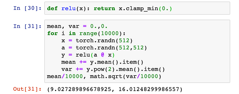
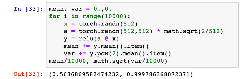
It turns out that when using a ReLU activation, a single layer will, on average have standard deviation that’s very close to the square root of the number of input connections, divided by the square root of two, or √512/√2 in our example.

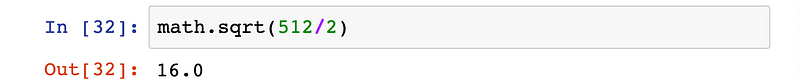
Scaling the values of the weight matrix a by this number will cause each individual ReLU layer to have a standard deviation of 1 on average.

As we showed before, keeping the standard deviation of layers’ activations around 1 will allow us to stack several more layers in a deep neural network without gradients exploding or vanishing.

This exploration into how to best initialize weights in networks with ReLU-like activations is what motivated Kaiming He et. al. to propose their own initialization scheme that’s tailored for deep neural nets that use these kinds of asymmetric, non-linear activations.

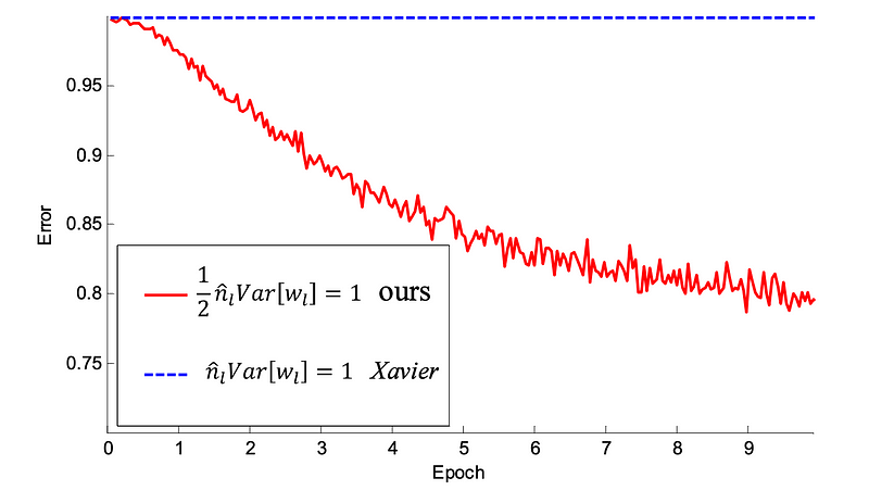
In their 2015 paper, He et. al. demonstrated that deep networks (e.g. a 22-layer CNN) would converge much earlier if the following input weight initialization strategy is employed:

1. Create a tensor with the dimensions appropriate for a weight matrix at a given layer, and populate it with numbers randomly chosen from a standard normal distribution.
2. Multiply each randomly chosen number by √2/√n where n is the number of incoming connections coming into a given layer from the previous layer’s output (also known as the “fan-in”).
3. Bias tensors are initialized to zero.

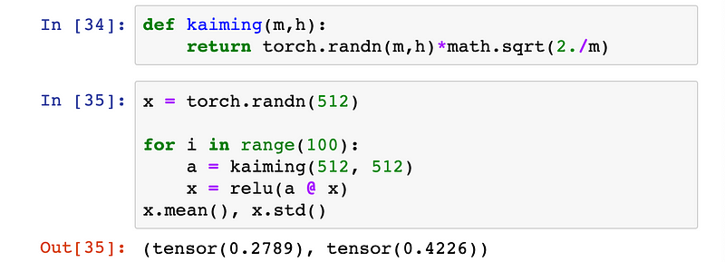
We can follow these directions to implement our own version of Kaiming initialization and verify that it can indeed prevent activation outputs from exploding or vanishing if ReLU is used at all layers of our hypothetical 100-layer network.

As a final comparison, here’s what would happen if we were to use Xavier initialization, instead.

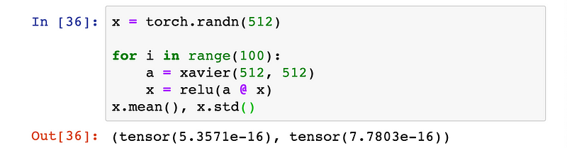
Ouch! When using Xavier to initialize weights, activation outputs have almost completely vanished by the 100th layer!

Incidentally, when they trained even deeper networks that used ReLUs, He et. al. found that a 30-layer CNN using Xavier initialization stalled completely and didn’t learn at all. However, when the same network was initialized according to the three-step procedure outlined above, it enjoyed substantially greater convergence.

Convergence of a 30-layer CNN thanks to Kaiming init. Credit: He et. al.

The moral of the story for us is that any network we train from scratch, especially for computer vision applications, will almost certainly contain ReLU activation functions and be several layers deep. In such cases, Kaiming should be our go-to weight init strategy.

Yes, You Too Can Be a Researcher

Even more importantly, I’m not ashamed to admit that I felt intimidated when I saw the Xavier and Kaiming formulas for the first time. What with their respective square roots of six and two, part of me couldn’t help but feel like they must have been the result of some sort of oracular wisdom I couldn’t hope to fathom on my own. And let’s face it, sometimes the math in deep learning papers can look a lot like hieroglyphics, except with no Rosetta Stone to aid in translation.

But I think the journey we took here showed us that this knee-jerk response of feeling of intimidated, while wholly understandable, is by no means unavoidable. Although the Kaiming and (especially) the Xavier papers do contain their fair share of math, we saw firsthand how experiments, empirical observation, and some straightforward common sense were enough to help derive the core set of principals underpinning what is currently the most widely-used weight initialization scheme.

Alternately put: when in doubt, be courageous, try things out, and see what happens!