3 Machine Learning Books that Helped me Level Up as a Data Scientist

http://www.datastuff.tech/data-science/3-machine-learning-books-that-helped-me-level-up-as-a-data-scientist/

Sumber :

Principles and Techniques of Data Science

https://www.textbook.ds100.org/
 
Data 8: Foundations of Data Science http://data8.org/fa16/
CS 88: Computational Structures in Data Science http://cs88-website.github.io/
CS 61A: Structure and Interpretation of Computer Programs https://cs61a.org/
DS100 Principles and Techniques of Data Science http://www.ds100.org/
Math 54, Linear Algebra and Differential Equations, Fall 2015https://math.berkeley.edu/~nadler/54fall2015.html
EE 16A | Designing Information Devices and Systems I  http://inst.eecs.berkeley.edu/~ee16a/fa16/
Stat89a: Linear Algebra for Data Science  https://www.stat.berkeley.edu/~mmahoney/s18-lads/

TextCaps : Handwritten Character Recognition with Very Small Datasets

https://twitter.com/hardmaru/status/1120863660107161600

Handwritten Character Recognition with Very Small Datasets They show that capsule networks can generate new training samples from existing ones, with realistic variations that are more human-like. They get 98.7% on MNIST with only 200 training samples. https://arxiv.org/abs/1904.08095 

How To Make Deep Learning Models That Don’t Suck

https://blog.nanonets.com/hyperparameter-optimization/



So you’ve watched all the tutorials. You now understand how a neural network works. You’ve built a cat and dog classifier. You tried your hand at a half-decent character-level RNN. You’re just one pip install tensorflow away from building the terminator, right? Wrong.

Source

A very important part of deep learning is finding the right hyperparameters. These are numbers that the model cannot learn.
In this article, I’ll walk you through some of the most common (and important) hyperparameters that you’ll encounter on your road to the #1 spot on the Kaggle leaderboards. In addition, I’ll also show you some powerful algorithms that can help you choose your hyperparameters wisely.

Hyperparameters in Deep Learning

Hyperparameters can be thought of as the tuning knobs of your model.
A fancy 7.1 Dolby Atmos home theatre system with a subwoofer that produces bass beyond the human ear’s audible range is useless if you set your AV receiver to stereo.

Photo by Michael Andree / Unsplash

Similarly, an inception_v3 with a trillion parameters won't even get you past MNIST if your hyperparameters are off.
So now, let's take a look at the knobs to tune before we get into how to dial in the right settings.

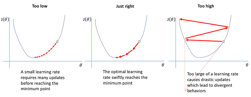
Learning Rate

Arguably the most important hyperparameter, the learning rate, roughly speaking, controls how fast your neural net “learns”.
So why don’t we just amp this up and live life on the fast lane?

Source

Not that simple. Remember, in deep learning, our goal is to minimize a loss function. If the learning rate is too high, our loss will start jumping all over the place and never converge.

Source

And if the learning rate is too small, the model will take way too long to converge, as illustrated above.

Momentum

Since this article focuses on hyperparameter optimization, I’m not going to explain the whole concept of momentum. But in short, the momentum constant can be thought of as the mass of a ball that’s rolling down the surface of the loss function.
The heavier the ball, the quicker it falls. But if it’s too heavy, it can get stuck or overshoot the target.

Source

Dropout

If you’re sensing a theme here, I’m now going to direct you to Amar Budhiraja’s article on dropout.

Source

But as a quick refresher, dropout is a regularization technique proposed by Geoff Hinton that randomly sets activations in a neural network to 0 with a probability of $p$. This helps prevent neural nets from overfitting (memorizing) the data as opposed to learning it.
$p$ is a hyperparameter.

Architecture — Number of Layers, Neurons Per Layer, etc.

Another (fairly recent) idea is to make the architecture of the neural network itself a hyperparameter.
Although we generally don’t make machines figure out the architecture of our models (otherwise AI researchers would lose their jobs), some new techniques like Neural Architecture Search have been implemented this idea with varying degrees of success.
If you’ve heard of AutoML, this is basically how Google does it: make everything a hyperparameter and then throw a billion TPUs at the problem and let it solve itself.
But for the vast majority of us who just want to classify cats and dogs with a budget machine cobbled together after a Black Friday sale, it’s about time we figured out how to make those deep learning models actually work.

Hyperparameter Optimization Algorithms

Grid Search

This is the simplest possible way to get good hyperparameters. It’s literally just brute force.
The Algorithm: Try out a bunch of hyperparameters from a given set of hyperparameters, and see what works best.
Try it in a notebookThe Pros: It’s easy enough for a fifth grader to implement. Can be easily parallelized.
The Cons: As you probably guessed, it’s insanely computationally expensive(as all brute force methods are).
Should I use it: Probably not. Grid search is terribly inefficient. Even if you want to keep it simple, you’re better off using random search.

Random Search

It’s all in the name — random search searches. Randomly.
The Algorithm: Try out a bunch of random hyperparameters from a uniform distribution over some hyperparameter space, and see what works best.
Try it in a notebookThe Pros: Can be easily parallelized. Just as simple as grid search, but a bit better performance, as illustrated below:

Source

The Cons: While it gives better performance than grid search, it is still just as computationally intensive.
Should I use it: If trivial parallelization and simplicity are of utmost importance, go for it. But if you can spare the time and effort, you'll be rewarded big time by using Bayesian Optimization.

Bayesian Optimization

Unlike the other methods we’ve seen so far, Bayesian optimization uses knowledge of previous iterations of the algorithm. With grid search and random search, each hyperparameter guess is independent. But with Bayesian methods, each time we select and try out different hyperparameters, the inches toward perfection.

Source

The ideas behind Bayesian hyperparameter tuning are long and detail-rich. So to avoid too many rabbit holes, I’ll give you the gist here. But be sure to read up on Gaussian processes and Bayesian optimization in general, if that’s the sort of thing you’re interested in.
Remember, the reason we’re using these hyperparameter tuning algorithms is that it’s infeasible to actually evaluate multiple hyperparameter choices individually. For example, let’s say we wanted to find a good learning rate manually. This would involve setting a learning rate, training your model, evaluating it, selecting a different learning rate, training you model from scratch again, re-evaluating it, and the cycle continues.
The problem is, “training your model” can take up to days (depending on the complexity of the problem) to finish. So you would only be able to try a few learning rates by the time the paper submission deadline for the conference turns up. And what do you know, you haven’t even started playing with the momentum. Oops.

Photo by Brad Neathery / Unsplash

The Algorithm: Bayesian methods attempt to build a function (more accurately, a probability distribution over possible function) that estimates how good your model might be for a certain choice of hyperparameters. By using this approximate function (called a surrogate function in literature), you don’t have to go through the set, train, evaluate loop too many time, since you can just optimize the hyperparameters to the surrogate function.
As an example, say we want to minimize this function (think of it like a proxy for your model's loss function):

The surrogate function comes from something called a Gaussian process (note: there are other ways to model the surrogate function, but I’ll use a Gaussian process). Like, I mentioned, I won’t be doing any math heavy derivations, but here’s what all that talk about Bayesians and Gaussians boils down to:
$\mathbb{P} (F_n(X)|X_n) = \frac{e^{-\frac12 F_n^T \Sigma_n^{-1} F_n}}{\sqrt{(2\pi)^n |\Sigma_n|}}$
​e−21​FnT​Σn−1​Fn​​
Which, admittedly is a mouthful. But let’s try to break it down.
The left-hand side is telling you that a probability distribution is involved (given the presence of the fancy looking $\mathbb{P}$ ). Looking inside the brackets, we can see that it’s a probability distribution of $F_n(X)$, which is some arbitrary function. Why? Because remember, we’re defining a probability distribution over allpossible functions, not just a particular one. In essence, the left-hand side says that the probability that the true function that maps hyperparameters to the model’s metrics (like validation accuracy, log likelihood, test error rate, etc.) is $F_n(X)$, given some sample data $X_n$ is equal to whatever’s on the right-hand side.
Now that we have the function to optimize, we optimize it.
Here's what the Gaussian process will look like before we start the optimization process:

Gaussan process before iteration with 2 points

Use your favorite optimizer of choice (the pros like maximizing expected improvement), but somehow, just follow the signs (or gradients) and before you know it, you’ll end up at your local minima.
After a few iterations, the Gaussian process gets better at approximating the target function:

Gaussan process after 3 iteration with 2 points

Regardless of the method you used, you have now found the `argmin` of the surrogate function. Ans surprise, surprise, those arguments that minimize the surrogate function are (an estimate of) the optimal hyperparameters! Yay.
The final result should look like this:

Gaussan process after 7 iteration with 2 points

Use these “optimal” hyperparameters to do a training run on your neural net, and you should see some improvement. But you can also use this new information to redo the whole Bayesian optimization process, again, and again, and again. Feel free to run the Bayesian loop however many times you want, but be wary. You are actually computing stuff. Those AWS credits don’t come for free, you know. Or do they…
Try it in a notebookThe Pros: Bayesian optimization gives better results than both grid search and random search.
The Cons: It's not as easy to parallelize.
Should I Use It: In most cases, yes! The only exceptions would be if

• You're a deep learning expert and you don't need the help of a measly approximation algorithm.
• You have access to a vast computational resources and can massively parallelize grid search and random search.
• If you're an frequentist/anti-Bayesian statistics nerd.

An Alternate Approach To Finding A Good Learning Rate

In all the methods we’ve seen so far, there’s one underlying theme: automate the job of the machine learning engineer. Which is great and all; until your boss gets wind of this and decides to replace you with 4 RTX Titan cards. Huh. Guess you should have stuck to manual search.

Photo by Rafael Pol / Unsplash

But do not despair, there is active research in the field of making researchers do less and simultaneously get paid more. And one of the ideas that has worked extremely well is the learning rate range test, which, to the best of my knowledge, first appeared in a paper by Leslie Smith.
The paper is actually about a method for scheduling (changing) the learning rate over time. The LR (learning rate) range test was a gold nugget that the author just casually dropped on the side.
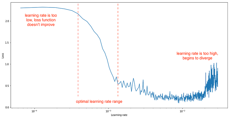
When you’re using a learning rate schedule that varies the learning rate from a minimum to maximum value, such as cyclic learning rates or stochastic gradient descent with warm restarts, the author suggests linearly increasing the learning rate after each iteration from a small to a large value (say, 1e-7 to 1e-1), evaluate the loss at each iteration, and plot the loss (or test error or accuracy) against the learning rate on a log scale. Your plot should look something like this:

Source

Try it in a notebookAs marked on the plot, you’d then use set your learning rate schedule to bounce between the minimum and maximum learning rate, which are found by looking at the plot and trying to eyeball the region with the steepest gradient.
Here's a sample LR range test plot (DenseNet trained on CIFAR10) from our Colab notebook:

Sample LR range test from DenseNet 201 trained on CIFAR10

As a rule of thumb, if you’re not doing any fancy learning rate schedule stuff, just set your constant learning rate to an order of magnitude lower than the minimum value on the plot. In this case that would be roughly 1e-2.
The coolest part about this method, other than that it works really well and spares you the time, mental effort, and compute required to find good hyperparameters with other algorithms, is that it costs virtually no extra compute.
While the other algorithms, namely grid search, random search, and Bayesian Optimization, require you to run a whole project tangential to your goal of training a good neural net, the LR range test is just executing a simple, regular training loop, and keeping track of a few variables along the way.
Here's the type of convergence speed you can expect when using a optimal learning rate (from the example in the notebook):

Loss vs. Batches for a model fit with the optimal learning rate

The LR range test has been implemented by the team at fast.ai, and you should definitely take a look at their library to implement the LR range test (they call it the learning rate finder) as well as many other algorithms with ease.

For The More Sophisticated Deep Learning Practitioner

If you're interested, there's also a notebook written in pure pytorch that implements the above.  This might give you a better understanding of the behind-the-scenes training process. Check it out here.

Save Yourself The Effort

Of course, all these algorithms, as great as they are, don’t always work in practice. There are many more factors to consider when training neural nets, such as how you’re going to preprocess your data, define your model, and actually get a computer powerful enough to run the darn thing.
Nanonets provides easy to use APIs to train and deploy custom deep learning models. It takes care of all of the heavy lifting, including data augmentation, transfer learning and yes, hyperparameter optimization!
Nanonets makes use of Bayesian search on their vast GPU clusters to find the right set of hyperparameters without the need for you to worry about blowing cash on the latest graphics card and out of bounds for axis 0.
Once it finds the best model, Nanonets serves it on their cloud for you to test the model using their web interface or to integrate it into your program using 2 lines of code.
Say goodbye to less than perfect models.

Conclusion

In this article, we’ve talked about hyperparameters and a few methods of optimizing them. But what does it all mean?
As we try harder and harder to democratize AI technology, automated hyperparameter tuning is probably a step in the right direction. It allows regular folks like you and me to build amazing deep learning applications without a math PhD.
While you could argue that making model hungry for computing power leaves the very best models in the hands of those that can afford said computing power, cloud services like AWS and Nanonets help democratize access to powerful machines, making deep learning far more accessible.
But more fundamentally, what we’re actually doing here using math to solve more math. Which is interesting not only because of how meta that sounds, but also because of how easily it can be misinterpreted.

Source

We certainly have come a long way from the era of punch cards and trace tables to an age where we optimize functions that optimize functions that optimize functions. But we are nowhere close to building machines that can "think" on their own.

---

And that's not discouraging, not in the least, because if humanity can do so much with so little, imagine what the future holds, when our visions become something that we can actually see.
And so we sit, on a cushioned mesh chair staring at a blank terminal screen, every keystroke giving us a sudo superpower that can wipe the disk clean.
And so we sit, we sit there all day, because the next big breakthrough might be just one pip install away.

Introduction to Anomaly Detection in Python

https://blog.floydhub.com/introduction-to-anomaly-detection-in-python/

There are always some students in a classroom who either outperform the other students or failed to even pass with a bare minimum when it comes to securing marks in subjects. Most of the times, the marks of the students are generally normally distributed apart from the ones just mentioned. These marks can be termed as extreme highs and extreme lows respectively. In Statistics and other related areas like Machine Learning, these values are referred to as Anomalies or Outliers.

The very basic idea of anomalies is really centered around two values - extremely high values and extremely low values. Then why are they given importance? In this article, we will try to investigate questions like this. We will see how they are created/generated, why they are important to consider while developing machine learning models, how they can be detected. We will also do a small case study in Python to even solidify our understanding of anomalies. But before we get started let’s take some concrete example to understand how anomalies look like in the real world.

A dive into the wild: Anomalies in the real world

Suppose, you are a credit card holder and on an unfortunate day it got stolen. Payment Processor Companies (like PayPal) do keep a track of your usage pattern so as to notify in case of any dramatic change in the usage pattern. The patterns include transaction amounts, the location of transactions and so on. If a credit card is stolen, it is very likely that the transactions may vary largely from the usual ones. This is where (among many other instances) the companies use the concepts of anomalies to detect the unusual transactions that may take place after the credit card theft. But don’t let that confuse anomalies with noise. Noise and anomalies are not the same. So, how noise looks like in the real world?
Let’s take the example of the sales record of a grocery shop. People tend to buy a lot of groceries at the start of a month and as the month progresses the grocery shop owner starts to see a vivid decrease in the sales. Then he starts to give discounts on a number of grocery items and also does not fail to advertise about the scheme. This discount scheme might cause an uneven increase in sales but are they normal? They, sure, are not. These are noises (more specifically stochastic noises).
By now, we have a good idea of how anomalies look like in a real-world setting. Let’s now describe anomalies in data in a bit more formal way.

Find the odd ones out: Anomalies in data

Allow me to quote the following from classic book Data Mining. Concepts and Techniques by Han et al. -

Outlier detection (also known as anomaly detection) is the process of finding data objects with behaviors that are very different from expectation. Such objects are called outliers or anomalies.

Could not get any better, right? To be able to make more sense of anomalies, it is important to understand what makes an anomaly different from noise.
The way data is generated has a huge role to play in this. For the normal instances of a dataset, it is more likely that they were generated from the same process but in case of the outliers, it is often the case that they were generated from a different process(s).

Some points (including the odd ones) on a 2D-plane

In the above figure, I show you what it is like to be outliers within a set of closely related data-points. The closeness is governed by the process that generated the data points. From this, it can be inferred that the process for generated those two encircled data-points must have been different from that one that generated the other ones. But how do we justify that those red data points were generated by some other process? Assumptions!
While doing anomaly analysis, it is a common practice to make several assumptions on the normal instances of the data and then distinguish the ones that violate these assumptions. More on these assumptions later!
The above figure may give you a notion that anomaly analysis and cluster analysis may be the same things. They are very closely related indeed, but they are not the same! They vary in terms of their purposes. While cluster analysis lets you group similar data points, anomaly analysis lets you figure out the odd ones among a set of data points.
We saw how data generation plays a crucial role in anomaly detection. So, it will be worth enough to discuss what might lead towards the creation of anomalies in data.

Generation of anomalies in data

The way anomalies are generated hugely varies from domain to domain, application to application. Let’s take a moment to review some of the fields where anomaly detection is extremely vital -

• Intrusion detection systems - In the field of computer science, unusual network traffic, abnormal user actions are common forms of intrusions. These intrusions are capable enough to breach many confidential aspects of an organization. Detection of these intrusions is a form of anomaly detection.
• Fraud detection in transactions - One of the most prominent use cases of anomaly detection. Nowadays, it is common to hear about events where one’s credit card number and related information get compromised. This can, in turn, lead to abnormal behavior in the usage pattern of the credit cards. Therefore, to effectively detect these frauds, anomaly detection techniques are employed.
• Electronic sensor events - Electronic sensors enable us to capture data from various sources. Nowadays, our mobile devices are also powered with various sensors like light sensors, accelerometer, proximity sensors, ultrasonic sensors and so on. Sensor data analysis has a lot of interesting applications. But what happens when the sensors become ineffective? This shows up in the data they capture. When a sensor becomes dysfunctional, it fails to capture the data in the correct way and thereby produces anomalies.  Sometimes, there can be abnormal changes in the data sources as well. For example, one’s pulse rate may get abnormally high due to several conditions and this leads to anomalies. This point is also very crucial considering today’s industrial scenario. We are approaching and embracing Industry 4.0 in which IoT (Internet of Things) and AI (Artificial Intelligence) are integral parts. When there is IoT, there are sensors. In fact a wide network of sensors, catering to an arsenal of real-world problems. When these sensors start to behave inconsistently the signals they convey get also uncanny, thereby causing unprecedented troubleshooting. Hence, systematic anomaly detection is a must here.

and more.
In all of the above-mentioned applications, the general idea of normal and abnormal data-points is similar. Abnormal ones are those which deviate hugely from the normal ones. These deviations are based on the assumptions that are taken while associating the data points to normal group. But then again, there are more twists to it i.e. the types of the anomalies.

It is now safe enough to say that data generation and data capturing processes are directly related to anomalies in the data and it varies from application to application.

Anomalies can be of different types

In the data science literature, anomalies can be of the three types as follows. Understanding these types can significantly affect the way of dealing with anomalies.

• Global
• Contextual
• Collective

In the following subsections, we are to take a closer look at each of the above and discuss their key aspects like their importance, grounds where they should be paid importance to.

Global anomalies

Global anomalies are the most common type of anomalies and correspond to those data points which deviate largely from the rest of the data points. The figure used in the “Find the odd ones out: Anomalies in data” section actually depicts global anomalies.

Global anomalies

A key challenge in detecting global anomalies is to figure out the exact amount of deviation which leads to a potential anomaly. In fact, this is an active field of research. Follow this excellent paper by Macha et al. for more on this. Global anomalies are quite often used in the transnational auditing systems to detect fraud transactions. In this case, specifically, global anomalies are those transactions which violate the general regulations.
You might be thinking that the idea of global anomalies (deviation from the normal) may not always hold practical with respect to numerous conditions, context and similar aspects.  Yes, you are thinking just right. Anomalies can be contextual too!

Contextual anomalies

Consider today’s temperature to be 32 degrees centigrade and we are in Kolkata, a city situated in India. Is the temperature normal today? This is a highly relative question and demands for more information to be concluded with an answer. Information about the season, location etc. are needed for us to jump to give any response to the question - “Is the temperature normal today?”
Now, in India, specifically in Kolkata, if it is Summer, the temperature mentioned above is fine. But if it is Winter, we need to investigate further.  Let’s take another example. We all are aware of the tremendous climate change i.e. causing the Global Warming. The latest results are with us also. From the archives of The Washington Post:

Alaska just finished one of its most unusually warm Marches ever recorded. In its northern reaches, the March warmth was unprecedented.

Take note of the phrase “unusually warm”. It refers to 59-degrees Fahrenheit. But this may not be unusually warm for other countries. This unusual warmth is an anomaly here.
These are called contextual anomalies where the deviation that leads to the anomaly depends on contextual information. These contexts are governed by contextual attributes and behavioral attributes. In this example, location is a contextual attribute and temperature is a behavioral attribute.

Contextual anomalies in time-series data

The above figure depicts a time-series data over a particular period of time. The plot was further smoothed by kernel density estimation to present the boundary of the trend. The values have not fallen outside the normal global bounds, but there are indeed abnormal points (highlighted in orange) when compared to the seasonality.
While dealing with contextual anomalies, one major aspect is to examine the anomalies in various contexts. Contexts are almost always very domain specific. This is why in most of the applications that deal with contextual anomalies, domain experts are consulted to formalize these contexts.

Collective anomalies

In the following figure, the data points marked in green have collectively formed a region which substantially deviates from the rest of the data points.

Collective anomalies

This an example of a collective anomaly. The main idea behind collective anomalies is that the data points included in forming the collection may not be anomalies when considered individually. Let’s take the example of a daily supply chain in a textile firm. Delayed shipments are very common in industries like this. But on a given day, if there are numerous shipment delays on orders then it might need further investigation. The delayed shipments do not contribute to this individually but a collective summary is taken into account when analyzing situations like this.
Collective anomalies are interesting because here you do not only to look at individual data points but also analyze their behavior in a collective fashion.
So far, we have introduced ourselves to the basics of anomalies, its types and other aspects like how anomalies are generated in specific domains. Let’s now try to relate to anomalies from a machine learning specific context. Let’s find out answers to general questions like - why anomalies are important to pay attention to while developing a machine learning model and so on.

Machine learning & anomalies: Could it get any better?

The heart and soul of any machine learning model is the data that is being fed to it. Data can be of any form practically - structured, semi-structured and unstructured. Let’s go into these categories for now. At all their cores, machine learning models try to find the underlying patterns of the data that best represent them. These patterns are generally learned as mathematical functions and these patterns are used for making predictions, making inferences and so on. To this end, consider the following toy dataset:

A dummy dataset 

The dataset has two features: x1 and x2 and the predictor variable (or the label) is y. The dataset has got 6 observations. Upon taking a close look at the data points, the fifth data point appears to be the odd one out here. Really? Well, it depends on a few things -

• We need to take the domain into the account here. The domain to which the dataset belongs to. This is particularly important because until and unless we have information on that, we cannot really say if the fifth data point is an extreme one (anomaly). It might so happen that this set of values is possible in the domain.
• While the data was getting captured, what was the state of the capturing process? Was it functioning in the way it is expected to? We may not always have answers to questions like these. But they are worth considering because this can change the whole course of the anomaly detection process.

Now coming to the perspective of a machine learning model, let’s formalize the problem statement -

Given a set of input vectors x1 and x2 the task is to predict y.

The prediction task is a classification task. Say, you have trained a model M on this data and you got a classification accuracy of 96% on this dataset. Great start for a baseline model, isn’t it? You may not be able to come up with a better model than this for this dataset. Is this evaluation just enough? Well, the answer is no! Let’s now find out why.
When we know that our dataset consists of a weird data-point, just going by the classification accuracy is not correct. Classification accuracy refers to the percentage of the correct predictions made by the model. So, before jumping into a conclusion of the model’s predictive supremacy, we should check if the model is able to correctly classify the weird data-point. Although the importance of anomaly detection varies from application to application, still it is a good practice to take this part into account. So, long story made short, when a dataset contains anomalies, it may not always be justified to just go with the classification accuracy of a model as the evaluation criteria.

The illusion, that gets created by the classification accuracy score in situations described above, is also known as classification paradox.

So, when a machine learning model is learning the patterns of the data given to it, it may have a critical time figuring out these anomalies and may give unexpected results. A very trivial and naive way to tackle this is just dropping off the anomalies from the data before feeding it to a model. But what happens when in an application, detection of the anomalies (we have seen the examples of these applications in the earlier sections) is extremely important? Can’t the anomalies be utilized in a more systematic modeling process? Well, the next section deals with that.

Getting benefits from anomalies

When training machine learning models for applications where anomaly detection is extremely important,  we need to thoroughly investigate if the models are being able to effectively and consistently identify the anomalies. A good idea of utilizing the anomalies that may be present in the data is to train a model with the anomalies themselves so that the model becomes robust to the anomaly detection. So, on a very high level, the task becomes training a machine learning model to specifically identify anomalies and later the model can be incorporated in a broader pipeline of automation.
A well-known method to train a machine learning model for this purpose is Cost-Sensitive Learning.  The idea here is to associate a certain cost whenever a model identifies an anomaly. Traditional machine learning models do not penalize or reward the wrong or correct predictions that they make. Let’s take the example of a fraudulent transaction detection system. To give you a brief description of the objective of the model - to identify the fraudulent transactions effectively and consistently. This is essentially a binary classification task. Now, let’s see what happens when a model makes a wrong prediction about a given transaction. The model can go wrong in the following cases  -

• Either misclassify the legitimate transactions as the fraudulent ones

or

• Misclassify the fraudulent ones as the legitimate ones

Confusion matrix in a fraud transactions' detector

To be able to understand this more clearly, we need to take the cost (that is incurred by the authorities) associated with the misclassifications into the account. If a legitimate transaction is categorized as fraudulent, the user generally contacts the bank to figure out what went wrong and in most of the cases, the respective authority and the user come to a mutual agreement. In this case, the administrative cost of handling the matter is most likely to be negligible. Now, consider the other scenario - “Misclassify the fraudulent ones as the legitimate ones.” This can indeed lead to some serious concerns. Consider, your credit card has got stolen and the thief purchased (let’s assume he somehow got to know about the security pins as well) something worth an amount (which is unusual according to your credit limit). Further, consider, this transaction did not raise any alarm to the respective credit card agency. In this case, the amount (that got debited because of the theft) may have to be reimbursed by the agency.
In traditional machine learning models, the optimization process generally happens just by minimizing the cost for the wrong predictions as made by the models. So, when cost-sensitive learning is incorporated to help prevent this potential issue, we associate a hypothetical cost when a model identifies an anomaly correctly. The model then tries to minimize the net cost (as incurred by the agency in this case) instead of the misclassification cost.
(N.B.: All machine learning models try to optimize a cost function to better their performance.)

Effectiveness and consistency are very important in this regard because sometimes a model may be randomly correct in the identification of an anomaly. We need to make sure that the model performs consistently well on the identification of the anomalies.

Let’s take these pieces of understandings together and approach the idea of anomaly detection in a programmatic way.

A case study of anomaly detection in Python

We will start off just by looking at the dataset from a visual perspective and see if we can find the anomalies. You can follow the accompanying Jupyter Notebook of this case study here.

Let's first create a dummy dataset for ourselves. The dataset will contain just two columns:

• Name of the employees of an organization
• Salaries of those employees (in USD) within a range of 1000 to 2500 (Monthly)

For generating the names (and make them look like the real ones) we will use a Python library called Faker (read the documentation here). For generating salaries, we will use the good old numpy. After generating these, we will merge them in a pandas DataFrame. We are going to generate records for 100 employees. Let's begin.
Note: Synthesizing dummy datasets for experimental purposes is indeed an essential skill.

# Import the necessary packages
import pandas as pd
import numpy as np
import matplotlib.pyplot as plt

# Comment out the following line if you are using Jupyter Notebook
# %matplotlib inline
# Use a predefined style set
plt.style.use('ggplot')

# Import Faker
from faker import Faker
fake = Faker()

# To ensure the results are reproducible
fake.seed(4321)

names_list = []

fake = Faker()
for _ in range(100):
  names_list.append(fake.name())

# To ensure the results are reproducible
np.random.seed(7)

salaries = []
for _ in range(100):
    salary = np.random.randint(1000,2500)
    salaries.append(salary)

# Create pandas DataFrame
salary_df = pd.DataFrame(
    {'Person': names_list,
     'Salary (in USD)': salaries
    })

# Print a subsection of the DataFrame
print(salary_df.head())

Let's now manually change the salary entries of two individuals. In reality, this can actually happen for a number of reasons such as the data recording software may have got corrupted at the time of recording the respective data.

salary_df.at[16, 'Salary (in USD)'] = 23
salary_df.at[65, 'Salary (in USD)'] = 17

# Verify if the salaries were changed
print(salary_df.loc[16])
print(salary_df.loc[65])

We now have a dataset to proceed with. We will start off our experiments just by looking at the dataset from a visual perspective and see if we can find the anomalies.

Seeing is believing: Detecting anomalies just by seeing

Hint: Boxplots are great!
As mentioned in the earlier sections, the generation of anomalies within data directly depends on the generation of the data points itself. To simulate this, our approach is good enough to proceed. Let's now some basic statistics (like minimum value, maximum value, 1st quartile values etc.) in the form of a boxplot.
Boxplot, because we get the following information all in just one place that too visually:

A sample boxplot

# Generate a Boxplot
salary_df['Salary (in USD)'].plot(kind='box')
plt.show()

We get:

Notice the tiny circle point in the bottom. You instantly get a feeling of something wrong in there as it deviates hugely from the rest of the data. Now, you decide to look at the data from another visual perspective i.e. in terms of histograms.
How about histograms?

# Generate a Histogram plot
salary_df['Salary (in USD)'].plot(kind='hist')
plt.show()

The result is this plot:

In the above histogram plot also, we can see there's one particular bin that is just not right as it deviates hugely from the rest of the data (phrase repeated intentionally to put emphasis on the deviation part). We can also infer that there are only two employees for which the salaries seem to be distorted (look at the y-axis).
So what might be an immediate way to confirm that the dataset contains anomalies? Let's take a look at the minimum and maximum values of the column Salary (in USD).

# Minimum and maximum salaries
print('Minimum salary ' + str(salary_df['Salary (in USD)'].min()))
print('Maximum salary ' + str(salary_df['Salary (in USD)'].max()))

We get:

Minimum salary 17
Maximum salary 2498

Look at the minimum value. From the accounts department of this hypothetical organization, you got to know that the minimum salary of an employee there is $1000. But you found out something different. Hence, its worth enough to conclude that this is indeed an anomaly. Let's now try to look at the data from a different perspective other than just simply plotting it.
Note: Although our dataset contains only one feature (i.e. Salary (in USD)) that contains anomalies in reality, there can be a lot of features which will have anomalies in them. Even there also, these little visualizations will help you a lot.

Clustering based approach for anomaly detection

We have seen how clustering and anomaly detection are closely related but they serve different purposes. But clustering can be used for anomaly detection. In this approach, we start by grouping the similar kind of objects. Mathematically, this similarity is measured by distance measurement functions like Euclidean distance, Manhattan distance and so on. Euclidean distance is a very popular choice when choosing in between several distance measurement functions. Let's take a look at what Euclidean distance is all about.
An extremely short note on Euclidean distance
If there are n points on a two-dimensional space(refer the following figure) and their coordinates are denoted by(x_i, y_i), then the Euclidean distance between any two points((x1, y1) and(x2, y2)) on this space is given by:

Equation for Euclidean distance

Scatter plot of a few points a 2D-plane

We are going to use K-Means clustering which will help us cluster the data points (salary values in our case). The implementation that we are going to be using for KMeans uses Euclidean distance internally. Let's get started.

# Convert the salary values to a numpy array
salary_raw = salary_df['Salary (in USD)'].values

# For compatibility with the SciPy implementation
salary_raw = salary_raw.reshape(-1, 1)
salary_raw = salary_raw.astype('float64')

We will now import the kmeans module from scipy.cluster.vq. SciPy stands for Scientific Python and provides a variety of convenient utilities for performing scientific experiments. Follow its documentation here. We will then apply kmeans to salary_raw.

# Import kmeans from SciPy
from scipy.cluster.vq import kmeans
    
# Specify the data and the number of clusters to kmeans()
centroids, avg_distance = kmeans(salary_raw, 4)

In the above chunk of code, we fed the salary data points the kmeans(). We also specified the number of clusters to which we want to group the data points. centroids are the centroids generated by kmeans() and avg_distance is the averaged Euclidean distance between the data points fed and the centroids generated by kmeans().Let's assign the groups of the data points by calling the vq() method. It takes -

• The data points
• The centroid as generated by the clustering algorithm (kmeans() in our case)

It then returns the groups (clusters) of the data points and the distances between the data points and its nearest groups.

# Get the groups (clusters) and distances
groups, cdist = cluster.vq.vq(salary_raw, centroids)

Let's now plot the groups we have got.

plt.scatter(salary_raw, np.arange(0,100), c=groups)
plt.xlabel('Salaries in (USD)')
plt.ylabel('Indices')
plt.show()

The resultant plot looks like:

Can you point to the anomalies? I bet you can! So a few things to consider before you fit the data to a machine learning model:

• Investigate the data thoroughly - take a look at each of the features that the dataset contains and pay close attention to their summary statistics like mean, median.
• Sometimes, it is easy for the eyes to generate a number of useful plots of the different features of the dataset (as shown in the above). Because with the plots in front of you, you instantly get to know about the presence of the weird values which may need further investigation.
• See how the features are correlated to one another. This will in turn help you to select the most significant features from the dataset and to discard the redundant ones. More on feature correlations here.

The above method for anomaly detection is purely unsupervised in nature. If we had the class-labels of the data points, we could have easily converted this to a supervised learning problem, specifically a classification problem. Shall we extend this? Well, why not?

Anomaly detection as a classification problem

To be able to treat the task of anomaly detection as a classification task, we need a labeled dataset. Let's give our existing dataset some labels.
We will first assign all the entries to the class of 0 and then we will manually edit the labels for those two anomalies. We will keep these class labels in a column named class. The label for the anomalies will be 1 (and for the normal entries the labels will be 0).

# First assign all the instances to 
salary_df['class'] = 0

# Manually edit the labels for the anomalies
salary_df.at[16, 'class'] = 1
salary_df.at[65, 'class'] = 1

# Veirfy 
print(salary_df.loc[16])

Let's take a look at the dataset again!
salary_df.head()

We now have a binary classification task. We are going to use proximity-based anomaly detection for solving this task. The basic idea here is that the proximity of an anomaly data point to its nearest neighboring data points largely deviates from the proximity of the data point to most of the other data points in the data set. Don't worry if this does not ring a bell now. Once, we visualize this, it will be clear.
We are going to use the k-NN classification method for this. Also, we are going to use a Python library called PyOD which is specifically developed for anomaly detection purposes.
I really encourage you to take a look at the official documentation of PyOD here.

# Importing KNN module from PyOD
from pyod.models.knn import KNN

The column Person is not at all useful for the model as it is nothing but a kind of identifier. Let's prepare the training data accordingly.

# Segregate the salary values and the class labels 
X = salary_df['Salary (in USD)'].values.reshape(-1,1)
y = salary_df['class'].values

# Train kNN detector
clf = KNN(contamination=0.02, n_neighbors=5)
clf.fit(X)

Let's discuss the two parameters we passed into KNN() -

• contamination - the amount of anomalies in the data (in percentage) which for our case is 2/100 = 0.02
• n_neighbors - number of neighbors to consider for measuring the proximity

Let's now get the prediction labels on the training data and then get the outlier scores of the training data. The outlier scores of the training data. The higher the scores are, the more abnormal. This indicates the overall abnormality in the data. These handy features make PyOD a great utility for anomaly detection related tasks.

# Get the prediction labels of the training data
y_train_pred = clf.labels_ 
    
# Outlier scores
y_train_scores = clf.decision_scores_

Let's now try to evaluate KNN() with respect to the training data. PyOD provides a handy function for this - evaluate_print().

# Import the utility function for model evaluation
from pyod.utils import evaluate_print

# Evaluate on the training data
evaluate_print('KNN', y, y_train_scores)

We get:
KNN ROC:1.0, precision @ rank n:1.0
We see that the KNN() model was able to perform exceptionally good on the training data. It provides three metrics and their scores -

• ROC
• Precision along with a confidence rank

Note: While detecting anomalies, we almost always consider ROC and Precision as it gives a much better idea about the model's performance. We have also seen its significance in the earlier sections.
We don't have any test data. But we can generate a sample salary value, right?

# A salary of $37 (an anomaly right?)
X_test = np.array([[37.]])

Let's now test how if the model could detect this salary value as an anomaly or not.

# Check what the model predicts on the given test data point
clf.predict(X_test)

The output should be: array([1])
We can see the model predicts just right. Let's also see how the model does on a normal data point.

# A salary of $1256
X_test_abnormal = np.array([[1256.]])

# Predict
clf.predict(X_test_abnormal)

And the output: array([0])
The model predicted this one as the normal data point which is correct. With this, we conclude our case study of anomaly detection which leads us to the concluding section of this article.

Challenges, further studies and more

We now have reached to the final section of this article. We have introduced ourselves to the whole world of anomaly detection and several of its nuances. Before we wrap up, it would be a good idea to discuss a few compelling challenges that make the task of anomaly detection troublesome -

• Differentiating between normal and abnormal effectively: It gets hard to define the degree up to which a data point should be considered as normal. This is why the need for domain knowledge is needed here. Suppose, you are working as a Data Scientist and you asked to check the health (in terms of abnormality that may be present in the data) of the data that your organization has collected. For complexity, assume that you have not worked with that kind of data before. You are just notified about a few points regarding the data like the data source, the collection process and so on. Now, to effectively model a system to capture the abnormalities (if at all present) in this data you need to decide on a sweet spot beyond which the data starts to get abnormal.  You will have to spend a sufficient amount of time to understand the data itself to reach that point.
• Distinguishing between noise and anomaly: We have discussed this earlier as well. It is critical to almost every anomaly detection challenges in a real-world setting. There can be two types of noise that can be present in data - Deterministic Noise and Stochastic Noise. While the later can be avoided to an extent but the former cannot be avoided. It comes as second nature in the data. When the amount deterministic noise tends to be very high, it often reduces the boundary between the normal and abnormal data points. Sometimes, it so happens that an anomaly is considered as a noisy data point and vice versa. This can, in turn, change the whole course of the anomaly detection process and attention must be given while dealing with this.

Let’s now talk about how you can take this study further and sharpen your data fluency.

Taking things further

It would be a good idea to discuss what we did not cover in this article and these will be the points which you should consider studying further -

• Anomaly detection in time series data - This is extremely important as time series data is prevalent to a wide variety of domains. It also requires some different set of techniques which you may have to learn along the way. Here is an excellent resource which guides you for doing the same.
• Deep learning based methods for anomaly detection - There are sophisticated Neural Network architectures (such as Autoencoders) which actually help you model an anomaly detection problem effectively. Here’s an example. Then there are Generative models at your disposal. This an active field of research, however. You can follow this paper to know more about it.
• Other more sophisticated anomaly detection methods - In the case study section, we kept our focus on the detection of global anomalies. But there’s another world of techniques which are designed for the detection of contextual and collective anomalies. To study further on this direction, you can follow Chapter 12 of the classic book  Data Mining. - Concepts and Techniques (3rd Edition). There are also ensemble methods developed for the purpose of anomaly detection which have shown state-of-the-art performance in many use cases. Here’s the paper which seamlessly describes these methods.

This is where you can find a wide variety of datasets which are known to have anomalies present in them. You may consider exploring them to deepen your understanding of different kinds of data perturbations.

More anomaly detection resources

• Anomaly Detection Learning Resources - A GitHub repo maintained by Yue Zhao
• Outlier Detection for Temporal Data by Gupta et al.
• Outlier detection methods for detecting cheaters in mobile gaming by Andrew Patterson

We have come to an end finally. I hope you got to scratch the surface of the fantastic world of anomaly detection. By now you should be able to take this forward and build novel anomaly detectors. I will be waiting to see you then.

---

Thanks to Alessio of FloydHub for sharing his valuable feedback on the article. It truly helped me enhance the quality of the article’s content.  I am really grateful to the entire team of FloydHub for letting me run the accompanying notebook on their platform (which is truly a Heroku for deep learning).

---

About Sayak Paul
Sayak is a Data Science Instructor at DataCamp where he develops projects that depict real world problems. He goes by the motto of understanding complex things and help people understand them as easily as possible. Sayak is an extensive blogger and all of his blogs can be found here. He is also working with his friends on the application of deep learning in Phonocardiogram classification. Sayak is also a FloydHub AI Writer. He is always open to discussing novel ideas and taking them forward to implementations. You can connect with Sayak on LinkedIn and GitHub.

https://habr.com/en/post/447732/

Dog Breed Identifier: Full Cycle Development from Keras Program to Android App. on Play Market

• Java,
• Python,
• Artificial Intelligence,
• Image processing,
• Development for Android

With the recent progress in Neural Networks in general and image Recognition particularly, it might seem that creating an NN-based application for image recognition is a simple routine operation. Well, to some extent it is true: if you can imagine an application of image recognition, then most likely someone have already did something similar. All you need to do is to Google it up and to repeat.

However, there are still countless little details that… they are not insolvable, no. They simply take too much of your time, especially if you are a beginner. What would be of help is a step-by-step project, done right in front of you, start to end. A project that does not contain «this part is obvious so let's skip it» statements. Well, almost :)

In this tutorial we are going to walk through a Dog Breed Identifier: we will create and teach a Neural Network, then we will port it to Java for Android and publish on Google Play.

For those of you who want to see a end result, here is the link to NeuroDog App on Google Play.

Web site with my robotics: robotics.snowcron.com.
Web site with: NeuroDog User Guide.

A Knee MRI Dataset And Competition

https://stanfordmlgroup.github.io/competitions/mrnet/

What is the MRNet Dataset?

The MRNet dataset consists of 1,370 knee MRI exams performed at Stanford University Medical Center. The dataset contains 1,104 (80.6%) abnormal exams, with 319 (23.3%) ACL tears and 508 (37.1%) meniscal tears; labels were obtained through manual extraction from clinical reports. The dataset accompanies the publication of the MRNet work here.

Dataset Details

The most common indications for the knee MRI examinations in this study included acute and chronic pain, follow-up or preoperative evaluation, injury/trauma. Examinations were performed with GE scanners (GE Discovery, GE Healthcare, Waukesha, WI) with standard knee MRI coil and a routine non-contrast knee MRI protocol that included the following sequences: coronal T1 weighted, coronal T2 with fat saturation, sagittal proton density (PD) weighted, sagittal T2 with fat saturation, and axial PD weighted with fat saturation. A total of 775 (56.6%) examinations used a 3.0-T magnetic field; the remaining used a 1.5-T magnetic field. See our paper for more details.

Splits

The exams have been split into a training set (1,130 exams, 1,088 patients), a validation set (called tuning set in the paper) (120 exams, 111 patients), and a hidden test set (called validation set in the paper) (120 exams, 113 patients). To form the validation and tuning sets, stratified random sampling was used to ensure that at least 50 positive examples of each label (abnormal, ACL tear, and meniscal tear) were present in each set. All exams from each patient were put in the same split.

Leaderboard

The leaderboard reports the average AUC of the abnormality detection, ACL tear, and Meniscal tear tasks.

Rank	Date	Model	AUC
1	Jan 09, 2019	mrnet-baseline (ensemble) Stanford University	0.917

Competition

We are hosting a competition to encourage others to develop models for automated interpretation of knee MRs. Our test set (called internal validation set in the paper) has its ground truth set using the majority vote of 3 practicing board-certified MSK radiologists (years in practice 6–19 years, average 12 years). The MSK radiologists had access to all DICOM series, the original report and clinical history, and follow-up exams during interpretation.

How can I participate?

MRNet uses a hidden test set for official evaluation of models. Teams submit their executable code on Codalab, which is then run on a test set that is not publicly readable. Such a setup preserves the integrity of the test results.
Here's a tutorial walking you through official evaluation of your model. Once your model has been evaluated officially, your scores will be added to the leaderboard.

The Bias-Variance trade-off : Explanation and Demo

https://towardsdatascience.com/the-bias-variance-trade-off-explanation-and-demo-8f462f8d6326

The Bias-Variance trade-off is a basic yet important concept in the field of data science and machine learning. Often, we encounter statements like “simpler models have high bias and low variance whereas more complex or sophisticated models have low bias and high variance” or “high bias leads to under-fitting and high variance leads to over-fitting”. But what do bias and variance actually mean and how are they related to the accuracy and performance of a model?

In this article, I will explain the intuitive and mathematical meaning of bias and variance, show the mathematical relation between bias, variance and performance of a model and finally demo the effects of varying the model complexity on bias and variance through a small example.

Assumptions to start with

Bias and variance are statistical terms and can be used in varied contexts. However, in this article, they will be discussed in terms of an estimator which is trying to fit/explain/estimate some unknown data distribution.

Before we delve into the bias and variance of an estimator, let us assume the following :-

1. There is a data generator, Y = f(X) + ϵ, which is generating Data(X,Y), where ϵ is the added random gaussian noise, centered at origin with some standard deviation σ i.e. E[ϵ] = 0 and Var(ϵ) = σ² . Note that data can be sampled repetitively from the generator yielding different sample sets say Xᵢ , Yᵢ on iᵗʰ iteration.
2. We are trying to estimate(fit a curve) to the sample set we have available from the generator, using an estimator. An estimator usually is a class of models like Ridge regressor, Decision Tree or Support Vector Regressor etc. A class of models can be represented as g(X/θ) where θ are the parameters. For different values of θ, we get different models within that particular class of models and we try vary θ to find the best fitting model for our sample set.

Meaning of Bias and Variance

Bias of an estimator is the the “expected” difference between its estimates and the true values in the data. Intuitively, it is a measure of how “close”(or far) is the estimator to the actual data points which the estimator is trying to estimate. Notice that I have used the word “expected” which implies that the difference is being thought over keeping in mind that we will be doing this model training experiment (ideally)infinite number of times. Each of those models will be trained on different sample sets Xᵢ , Yᵢ of the true data resulting in their parameters taking different values of θ in a bid to explain/fit/estimate that particular sample best.

Eventually for some test point xₒ , the bias of this estimator g(X) can be mathematically written as :-

Bias[g(xₒ)] = E[g(xₒ)] − f(xₒ)

which is literally the difference between the expected value of an estimator at that point and the true value at that same point.

Naturally, an estimator will have high bias at a test point(and hence overall too, in the limit) if it does NOT wiggle or change too much when a different sample set of the data is thrown at it. This will usually be the case when an estimator does not have enough “capacity” to adequately fit the inherent data generating function. Therefore, simpler models have a higher bias compared to more sophisticated models.

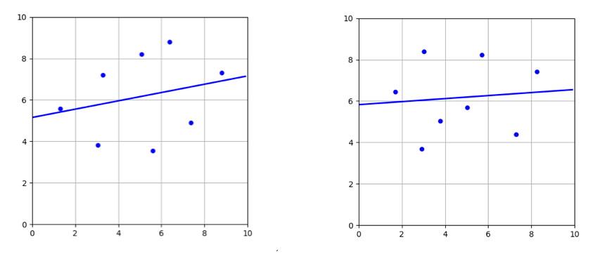
Hold these thoughts and we will come back to them again later in the article. For now, here is a figure to help solidify them a bit more.

Linear Regression fits for two different samples of size 8. Notice how curve has not changed too much although the sample sets are totally disjoint

Variance of an estimator is the “expected” value of the squared difference between the estimate of a model and the “expected” value of the estimate(over all the models in the estimator). Too convoluted to understand in a go? Lets break that sentence down..

Suppose we are training ∞ models using different sample sets of the data. Then at a test point xₒ, the expected value of the estimate over all those models is the E[g(xₒ)]. Also, for any individual model out of all the models, the estimate of that model at that point is g(xₒ). The difference between these two can be written as g(xₒ) − E[g(xₒ)]. Variance is the expected value of the square of this distance over all the models. Hence, variance of the estimator at at test point xₒ can be mathematically written as :-

Var[g(xₒ)] = E[(g(xₒ) − E[g(xₒ)])²]

Going by this equation, we can say that an estimator has high variance when the estimator “varies” or changes its estimate a lot at any data point, when it is trained over different sample sets of the data. 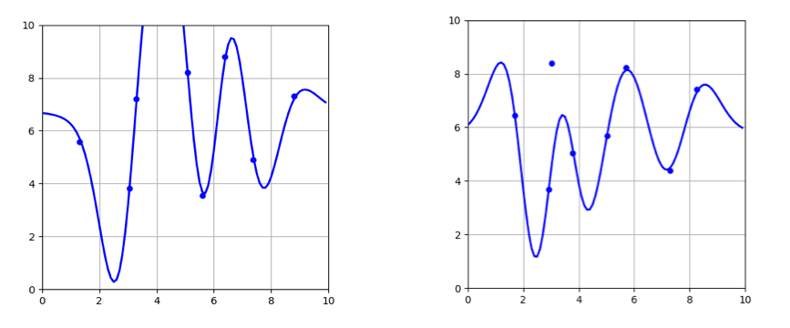Another way to put this is that the estimator is flexible/sophisticated enough, or has a high “capacity” to perfectly fit/explain/estimate the training sample set given to it due to which its value at other points fluctuates immensely.

Support Vector Regressor fits for the same sample sets. Notice how the curve changed drastically in this case. SVR is a high capacity estimator compared to Linear Regression hence higher variance

Notice that this interpretation of the meaning of high variance is exactly opposite to that of an estimator having high bias. This implies that bias and variance of an estimator are complementary to each other i.e. an estimator with high bias will vary less(have low variance) and an estimator with high variance will have less bias(as it can vary more to fit/explain/estimate the data points).

The Bias-Variance Decomposition

In this section, we see how the bias and variance of an estimator are mathematically related to each other and also to the performance of the estimator. We will start with defining estimator’s error at a test point as the “expected” squared difference between the true value and estimator’s estimate.

By now, it should be fairly clear that whenever we are talking about an expected value, we are referring to the expectation over all the possible models, trained individually over all the possible data samples from the data generator. For any unseen test point xₒ, we have :-

Err(xₒ) = E[(Y − g(xₒ))² | X = xₒ]

For notational simplicity, I am referring to f(xₒ) and g(xₒ) as f and g respectively and skipping the conditional on X :-

Err(xₒ) = E[(Y − g(xₒ))²]

= E[(f + ϵ − g)²]

= E[ϵ²] + E[(f − g)²] + 2.E[(f − g)ϵ]

= E[(ϵ − 0)²] + E[(f − E[g] + E[g] − g)²] + 2.E[fϵ] − 2.E[gϵ]

= E[(ϵ − E[ϵ])²] + E[(f − E[g] + E[g] − g)²] + 0 − 0

= Var(ϵ) + E[(g − E[g])²] + E[(E[g] − f)²] + 2.E[(g − E[g])(E[g] − f)]

= Var(ϵ) + Var(g) + Bias(g)² + 2.{E[g]² − E[gf] − E[g]² + E[gf]}

= σ² + Var(g) + Bias(g)²

1. So, the error(and hence the accuracy) of the estimator at an unseen data sample xₒ can be decomposed into variance of the noise in the data, bias and the variance of the estimator. This implies that both bias and variance are the sources of error of an estimator.
2. Also, in the previous section we have seen that bias and variance of an estimator are complementary to each other i.e. the increasing one of them would mean a decrease in the other and vice versa.

Now pause for a bit and try thinking a bit about what these two facts coupled together could mean for an estimator….

The Bias-Variance Trade-off

From the complementary nature of bias and variance and estimator’s error decomposing into bias and variance, it is clear that there is a trade-off between bias and variance when it comes to the performance of the estimator.

An estimator will have a high error if it has very high bias and low variance i.e. when it is not able to adapt at all to the data points in a sample set. On the other extreme, an estimator will also have a high error if it has very high variance and low bias i.e. when it adapts too well to all the data points in a sample set(a sample set is an incomplete representation of true data) and hence fails to generalize other unseen samples and eventually fails to generalize the true dataset.

An estimator that strikes a balance between the bias and variance is able to minimize the error better than those that live on extreme ends. Although it is beyond the scope of this article, this can be proved using basic differential calculus.

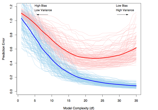
Courtesy : The Elements of Statistical Learning by Jerome H. Friedman, Robert Tibshirani, and Trevor Hastie. Blue curves show the training errors on 100 samples of size 50. Red curves are the corresponding test set errors

This figure has been taken from ESLR and it explains the trade-off very well. In this example, 100 sample sets of size 50 have been used to train 100 models of the same class, each of whose complexity/capacity is being increased from left to right. Each individual light blue curve belongs to a model and demonstrates how the model’s training set error changes as the complexity of the model is increased. Every point on the light red curve in turn is the model’s error on a common test set, tracing the curve as the complexity of the model is varied. Finally, the darker curves are the respective average(tending to expected value in the limit) training and test set errors. We can see that the models that strike a balance between bias and variance are able to generalize the best and perform substantially better than those with high bias or high variance.

Demo

I have put up a small demo showing everything I have talked about in this article. If all of this makes sense and you would like to try it out on your own, do check it out below! I have compared the bias-variance tradeoff between Ridge regressor and K-Nearest Neighbor Regressor with K = 1.

Keep in mind that KNN Regressor, K = 1 fits the training set perfectly so it “varies” a lot when the training set is changed while Ridge regressor does not.

Demo comparing bias-variance between KNN and Ridge Regressors

I hope this article explained the concept well and was fun to read! If you have any follow up questions, please post a comment and I will try to answer them.