A Tour of The Top 10 Algorithms for Machine Learning Newbies
In machine learning, there’s something called the “No Free Lunch”
theorem. In a nutshell, it states that no one algorithm works best for
every problem, and it’s especially relevant for supervised learning
(i.e. predictive modeling).
For
example, you can’t say that neural networks are always better than
decision trees or vice-versa. There are many factors at play, such as
the size and structure of your dataset.
As
a result, you should try many different algorithms for your problem,
while using a hold-out “test set” of data to evaluate performance and
select the winner.
Of
course, the algorithms you try must be appropriate for your problem,
which is where picking the right machine learning task comes in. As an
analogy, if you need to clean your house, you might use a vacuum, a
broom, or a mop, but you wouldn’t bust out a shovel and start digging.
The Big Principle
However, there is a common principle that underlies all supervised machine learning algorithms for predictive modeling.
Machine learning algorithms are described as learning a target function (f) that best maps input variables (X) to an output variable (Y): Y = f(X)
This
is a general learning task where we would like to make predictions in
the future (Y) given new examples of input variables (X). We don’t know
what the function (f) looks like or its form. If we did, we would use it
directly and we would not need to learn it from data using machine
learning algorithms.
The
most common type of machine learning is to learn the mapping Y = f(X)
to make predictions of Y for new X. This is called predictive modeling
or predictive analytics and our goal is to make the most accurate
predictions possible.
For
machine learning newbies who are eager to understand the basic of
machine learning, here is a quick tour on the top 10 machine learning
algorithms used by data scientists.
1 — Linear Regression
Linear regression is perhaps one of the most well-known and well-understood algorithms in statistics and machine learning.
Predictive
modeling is primarily concerned with minimizing the error of a model or
making the most accurate predictions possible, at the expense of
explainability. We will borrow, reuse and steal algorithms from many
different fields, including statistics and use them towards these ends.
The
representation of linear regression is an equation that describes a
line that best fits the relationship between the input variables (x) and
the output variables (y), by finding specific weightings for the input
variables called coefficients (B).
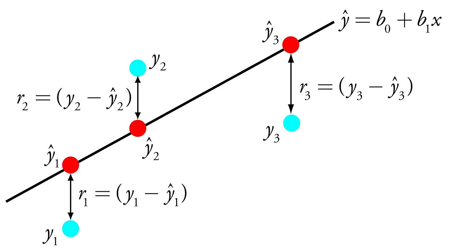
For example: y = B0 + B1 * x
We
will predict y given the input x and the goal of the linear regression
learning algorithm is to find the values for the coefficients B0 and B1.
Different
techniques can be used to learn the linear regression model from data,
such as a linear algebra solution for ordinary least squares and
gradient descent optimization.
Linear
regression has been around for more than 200 years and has been
extensively studied. Some good rules of thumb when using this technique
are to remove variables that are very similar (correlated) and to remove
noise from your data, if possible. It is a fast and simple technique
and good first algorithm to try.
2 — Logistic Regression
Logistic
regression is another technique borrowed by machine learning from the
field of statistics. It is the go-to method for binary classification
problems (problems with two class values).
Logistic
regression is like linear regression in that the goal is to find the
values for the coefficients that weight each input variable. Unlike
linear regression, the prediction for the output is transformed using a
non-linear function called the logistic function.
The
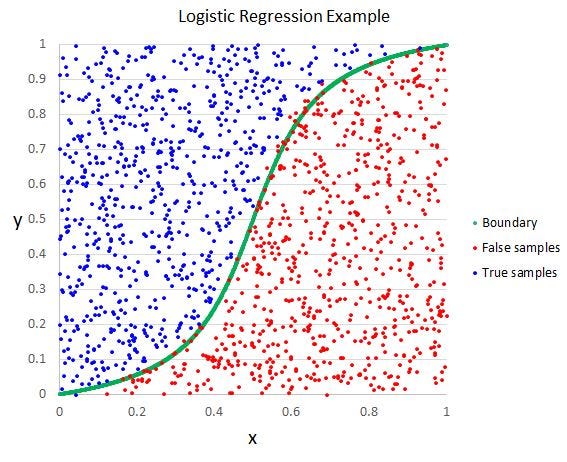
logistic function looks like a big S and will transform any value into
the range 0 to 1. This is useful because we can apply a rule to the
output of the logistic function to snap values to 0 and 1 (e.g. IF less
than 0.5 then output 1) and predict a class value.
Because
of the way that the model is learned, the predictions made by logistic
regression can also be used as the probability of a given data instance
belonging to class 0 or class 1. This can be useful for problems where
you need to give more rationale for a prediction.
Like
linear regression, logistic regression does work better when you remove
attributes that are unrelated to the output variable as well as
attributes that are very similar (correlated) to each other. It’s a fast
model to learn and effective on binary classification problems.
3 — Linear Discriminant Analysis
Logistic
Regression is a classification algorithm traditionally limited to only
two-class classification problems. If you have more than two classes
then the Linear Discriminant Analysis algorithm is the preferred linear
classification technique.
The
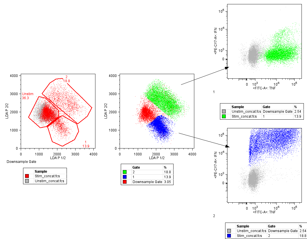
representation of LDA is pretty straight forward. It consists of
statistical properties of your data, calculated for each class. For a
single input variable this includes:
- The mean value for each class.
- The variance calculated across all classes.
Predictions
are made by calculating a discriminate value for each class and making a
prediction for the class with the largest value. The technique assumes
that the data has a Gaussian distribution (bell curve), so it is a good
idea to remove outliers from your data before hand. It’s a simple and
powerful method for classification predictive modeling problems.
4 — Classification and Regression Trees
Decision Trees are an important type of algorithm for predictive modeling machinelearning.
The
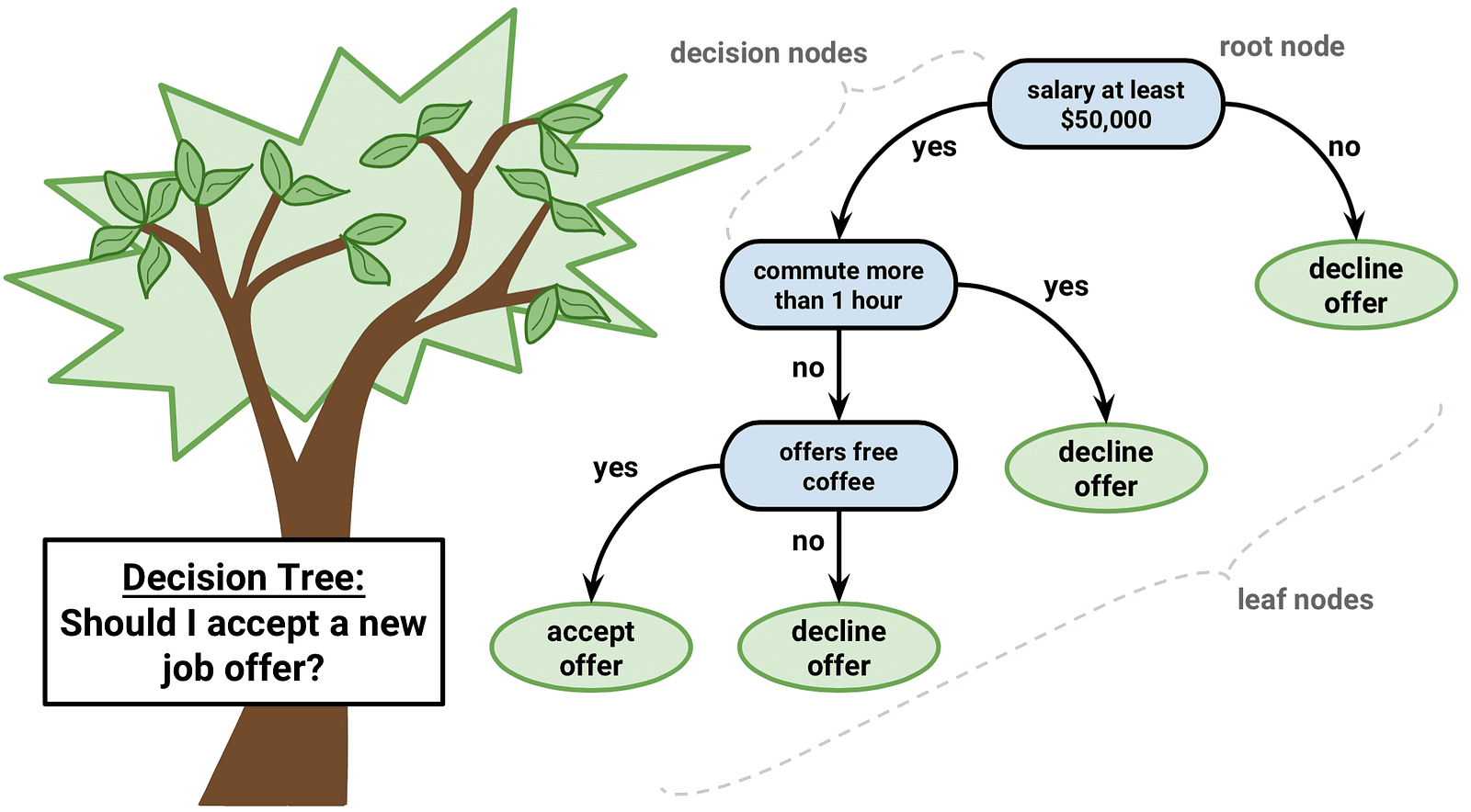
representation of the decision tree model is a binary tree. This is
your binary tree from algorithms and data structures, nothing too fancy.
Each node represents a single input variable (x) and a split point on
that variable (assuming the variable is numeric).
The
leaf nodes of the tree contain an output variable (y) which is used to
make a prediction. Predictions are made by walking the splits of the
tree until arriving at a leaf node and output the class value at that
leaf node.
Trees
are fast to learn and very fast for making predictions. They are also
often accurate for a broad range of problems and do not require any
special preparation for your data.
5 — Naive Bayes
Naive Bayes is a simple but surprisingly powerful algorithm for predictive modeling.
The
model is comprised of two types of probabilities that can be calculated
directly from your training data: 1) The probability of each class; and
2) The conditional probability for each class given each x value. Once
calculated, the probability model can be used to make predictions for
new data using Bayes Theorem. When your data is real-valued it is common
to assume a Gaussian distribution (bell curve) so that you can easily
estimate these probabilities.
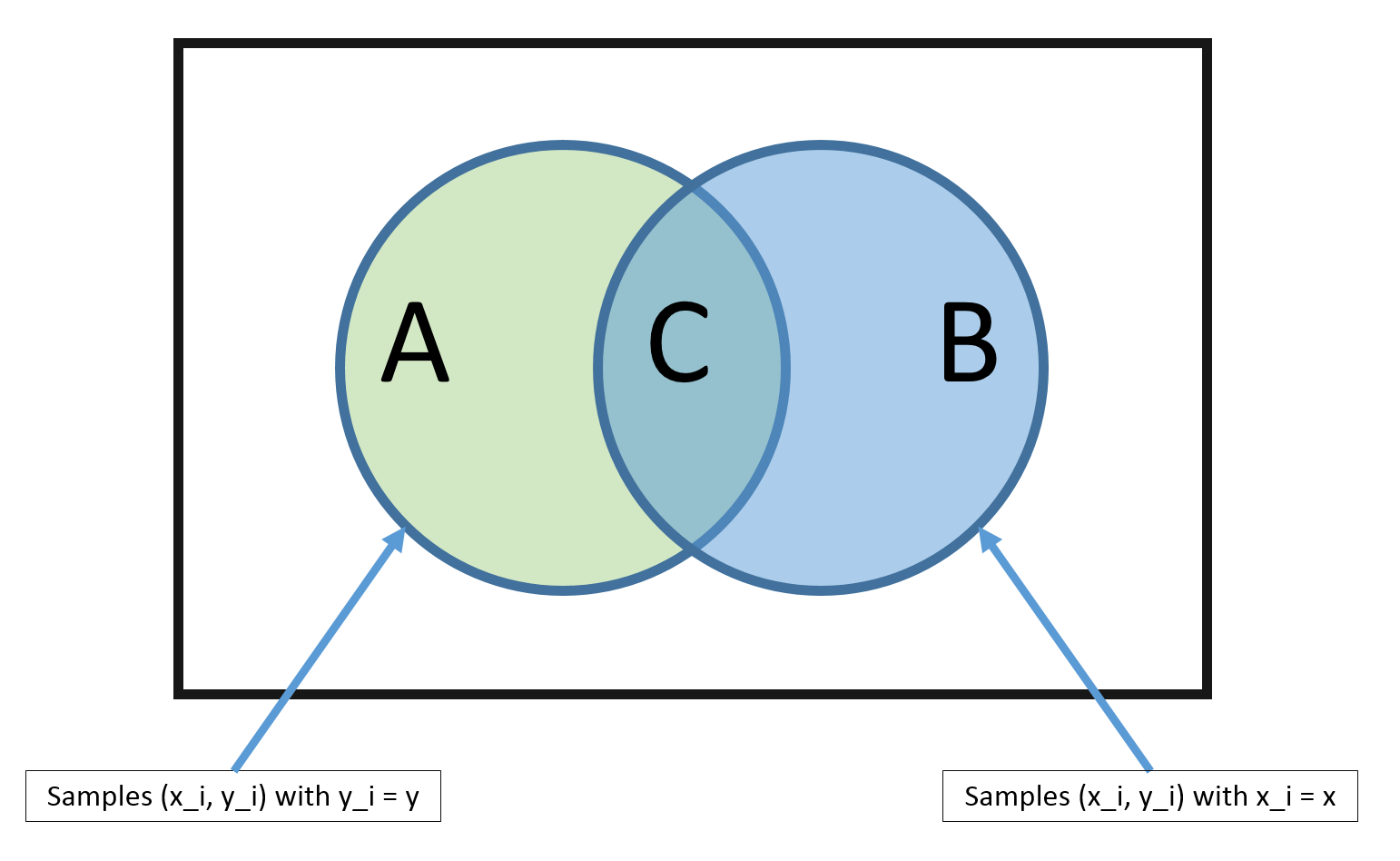
Naive
Bayes is called naive because it assumes that each input variable is
independent. This is a strong assumption and unrealistic for real data,
nevertheless, the technique is very effective on a large range of
complex problems.
6 — K-Nearest Neighbors
The
KNN algorithm is very simple and very effective. The model
representation for KNN is the entire training dataset. Simple right?
Predictions
are made for a new data point by searching through the entire training
set for the K most similar instances (the neighbors) and summarizing the
output variable for those K instances. For regression problems, this
might be the mean output variable, for classification problems this
might be the mode (or most common) class value.
The
trick is in how to determine the similarity between the data instances.
The simplest technique if your attributes are all of the same scale
(all in inches for example) is to use the Euclidean distance, a number
you can calculate directly based on the differences between each input
variable.
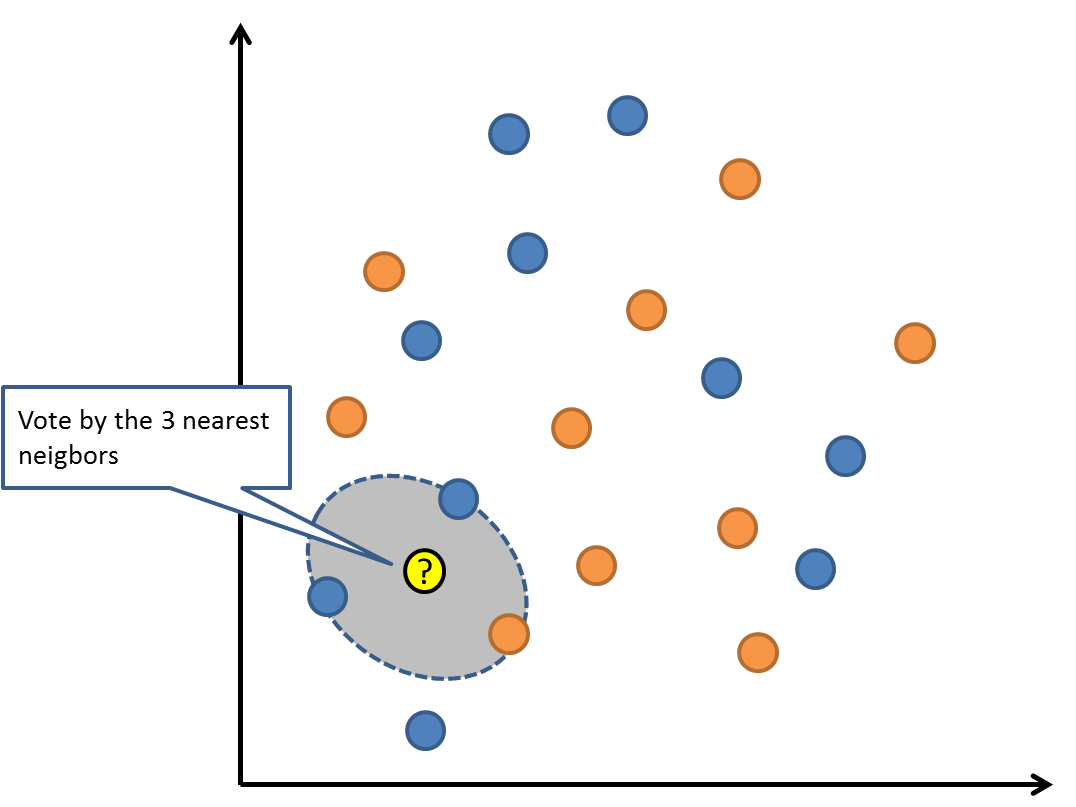
KNN
can require a lot of memory or space to store all of the data, but only
performs a calculation (or learn) when a prediction is needed, just in
time. You can also update and curate your training instances over time
to keep predictions accurate.
The
idea of distance or closeness can break down in very high dimensions
(lots of input variables) which can negatively affect the performance of
the algorithm on your problem. This is called the curse of
dimensionality. It suggests you only use those input variables that are
most relevant to predicting the output variable.
7 — Learning Vector Quantization
A
downside of K-Nearest Neighbors is that you need to hang on to your
entire training dataset. The Learning Vector Quantization algorithm (or
LVQ for short) is an artificial neural network algorithm that allows you
to choose how many training instances to hang onto and learns exactly
what those instances should look like.
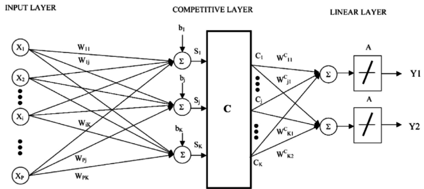
The
representation for LVQ is a collection of codebook vectors. These are
selected randomly in the beginning and adapted to best summarize the
training dataset over a number of iterations of the learning algorithm.
After learned, the codebook vectors can be used to make predictions just
like K-Nearest Neighbors. The most similar neighbor (best matching
codebook vector) is found by calculating the distance between each
codebook vector and the new data instance. The class value or (real
value in the case of regression) for the best matching unit is then
returned as the prediction. Best results are achieved if you rescale
your data to have the same range, such as between 0 and 1.
If
you discover that KNN gives good results on your dataset try using LVQ
to reduce the memory requirements of storing the entire training
dataset.
8 — Support Vector Machines
Support Vector Machines are perhaps one of the most popular and talked about machine learning algorithms.
A
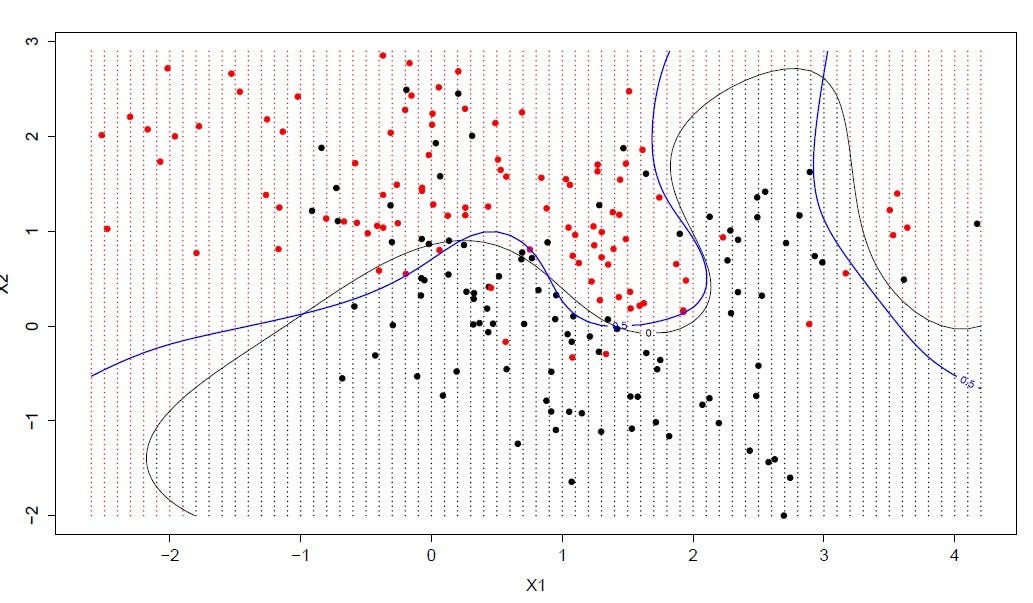
hyperplane is a line that splits the input variable space. In SVM, a
hyperplane is selected to best separate the points in the input variable
space by their class, either class 0 or class 1. In two-dimensions, you
can visualize this as a line and let’s assume that all of our input
points can be completely separated by this line. The SVM learning
algorithm finds the coefficients that results in the best separation of
the classes by the hyperplane.
The
distance between the hyperplane and the closest data points is referred
to as the margin. The best or optimal hyperplane that can separate the
two classes is the line that has the largest margin. Only these points
are relevant in defining the hyperplane and in the construction of the
classifier. These points are called the support vectors. They support or
define the hyperplane. In practice, an optimization algorithm is used
to find the values for the coefficients that maximizes the margin.
SVM might be one of the most powerful out-of-the-box classifiers and worth trying on your dataset.
9 — Bagging and Random Forest
Random
Forest is one of the most popular and most powerful machine learning
algorithms. It is a type of ensemble machine learning algorithm called
Bootstrap Aggregation or bagging.
The
bootstrap is a powerful statistical method for estimating a quantity
from a data sample. Such as a mean. You take lots of samples of your
data, calculate the mean, then average all of your mean values to give
you a better estimation of the true mean value.
In
bagging, the same approach is used, but instead for estimating entire
statistical models, most commonly decision trees. Multiple samples of
your training data are taken then models are constructed for each data
sample. When you need to make a prediction for new data, each model
makes a prediction and the predictions are averaged to give a better
estimate of the true output value.
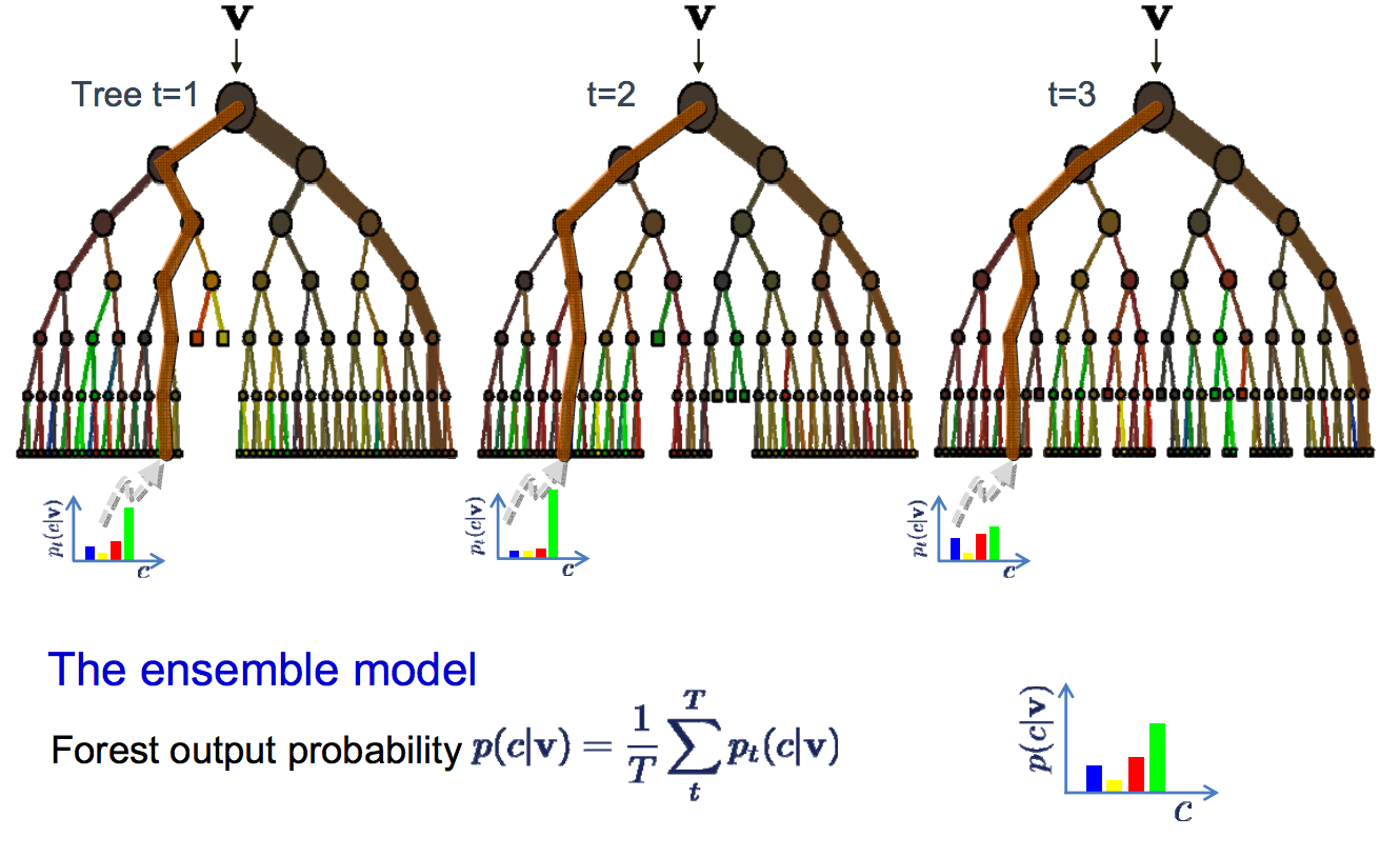
Random
forest is a tweak on this approach where decision trees are created so
that rather than selecting optimal split points, suboptimal splits are
made by introducing randomness.
The
models created for each sample of the data are therefore more different
than they otherwise would be, but still accurate in their unique and
different ways. Combining their predictions results in a better estimate
of the true underlying output value.
If
you get good results with an algorithm with high variance (like
decision trees), you can often get better results by bagging that
algorithm.
10 — Boosting and AdaBoost
Boosting
is an ensemble technique that attempts to create a strong classifier
from a number of weak classifiers. This is done by building a model from
the training data, then creating a second model that attempts to
correct the errors from the first model. Models are added until the
training set is predicted perfectly or a maximum number of models are
added.
AdaBoost
was the first really successful boosting algorithm developed for binary
classification. It is the best starting point for understanding
boosting. Modern boosting methods build on AdaBoost, most notably
stochastic gradient boosting machines.
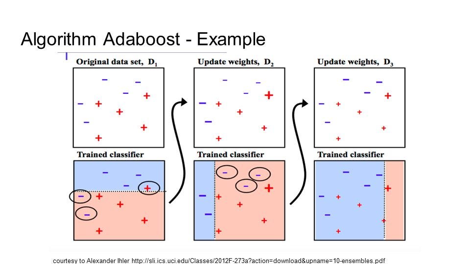
AdaBoost
is used with short decision trees. After the first tree is created, the
performance of the tree on each training instance is used to weight how
much attention the next tree that is created should pay attention to
each training instance. Training data that is hard to predict is given
more weight, whereas easy to predict instances are given less weight.
Models are created sequentially one after the other, each updating the
weights on the training instances that affect the learning performed by
the next tree in the sequence. After all the trees are built,
predictions are made for new data, and the performance of each tree is
weighted by how accurate it was on training data.
Because
so much attention is put on correcting mistakes by the algorithm it is
important that you have clean data with outliers removed.
Last Takeaway
A
typical question asked by a beginner, when facing a wide variety of
machine learning algorithms, is “which algorithm should I use?” The
answer to the question varies depending on many factors, including: (1)
The size, quality, and nature of data; (2) The available computational
time; (3) The urgency of the task; and (4) What you want to do with the
data.
Even
an experienced data scientist cannot tell which algorithm will perform
the best before trying different algorithms. Although there are many
other Machine Learning algorithms, these are the most popular ones. If
you’re a newbie to Machine Learning, these would be a good starting
point to learn.
— —
If you enjoyed this piece, I’d love it if you hit the clap button 👏 so others might stumble upon it. You can find my own code on GitHub, and more of my writing and projects at https://jameskle.com/. You can also follow me on Twitter, email me directly or find me on LinkedIn. Sign up for my newsletter to receive my latest thoughts on data science, machine learning, and artificial intelligence right at your inbox!
No comments:
Post a Comment