mages are nothing but a collection of pixel values and this idea was leveraged by the Computer scientist and researcher to build a Neural Network which is an analogy of the Human Brain and achieve exceptional results (sometimes even better than Human level accuracy).
Convolution Neural Networks are very similar to ordinary Neural Networks as they are made up of neurons that have learn-able weights and biases. Each neuron receives some inputs, performs a dot (scalar) product and optionally follows it with a non-linearity.
The whole network still expresses a single differentiable score
function, from the raw image pixels on one end to class scores at the
other. And they still have a loss function, to calculate relative
probability (e.g. SVM/Softmax) after the last (fully-connected) layer and all the tips/tricks developed for learning regular Neural Networks still apply.
In
recent times with the rise of data and computational power, ConvNets
have been extremely successful in identifying faces, different objects
and traffic signs apart from powering vision in robots and self driving
cars and a lot more.
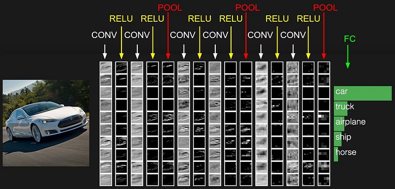
There are four main operations in the ConvNet as shown in Figure Below:
- Convolution
- Non Linearity (in this example ReLU)
- Pooling or Sub Sampling
- Classification
All Convolution Network: (https://arxiv.org/abs/1412.6806#)
Most
modern convolution neural networks (CNNs) used for object recognition
are built using the same principles: Alternating convolution and
max-pooling layers followed by a small number of fully connected layers.
Now in a recent paper it was noted that max-pooling can simply be
replaced by a convolution layer with an increased stride without loss in
accuracy on several image recognition benchmarks. Also the next
interesting thing mentioned in the paper was removing the Fully
Connected layer and put a Global Average pooling instead.
Removing
the Fully Connected layer may not seem that big of a surprise to
everybody, people have been doing the “no FC layers” thing for a long
time now. Yann LeCun even mentioned it on Facebook a while back — he has been doing it since the beginning.
Intuitively
this makes sense, the Fully connected network are nothing but
Convolution layers with the only difference is that the neurons in the
Convolution layers are connected only to a local region in the input,
and that many of the neurons in a Conv volume share parameters. However,
the neurons in both layers still compute dot products, so their
functional form is identical. Therefore, it turns out that it’s possible
to convert between FC and CONV layers and sometimes replace FC with
Conv layers
As
mentioned, the next thing is removing the spatial pooling operation
from the network, now this may raise few eyebrows. Let’s take a closer
look at this concept.
The
spatial Pooling (also called subsampling or downsampling) reduces the
dimensionality of each feature map but retains the most important
information.
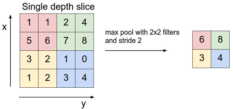
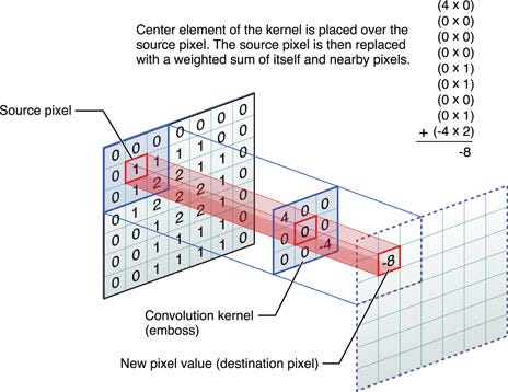
For
example, let’s consider Max Pooling. In case of Max Pooling, we define a
spatial window and take the largest element from the feature map within
that window. Now remember How Convolution works
(Fig. 2). Intuitively the convolution layer with higher strides can
serve as subsampling and downsampling layer it can make the input
representations smaller and more manageable. Also it can reduce the
number of parameters and computations in the network, therefore,
controlling things like overfitting.
To
reduce the size of the representation using larger stride in CONV layer
once in a while can always be a preferred option in many cases.
Discarding pooling layers has also been found to be important in
training good generative models, such as variational autoencoders (VAEs) or generative adversarial networks (GANs). Also it seems likely that future architectures will feature very few to no pooling layers.
Considering all of the above tips and tweaks, we have published a Keras model implementing the All Convolutional Network on Github.
- Importing the libraries and the dependencies
from __future__ import print_function
import tensorflow as tf
from keras.datasets import cifar10
from keras.preprocessing.image import ImageDataGenerator
from keras.models import Sequential
from keras.layers import Dropout, Activation, Convolution2D, GlobalAveragePooling2D
from keras.utils import np_utils
from keras.optimizers import SGD
from keras import backend as K
from keras.models import Model
from keras.layers.core import Lambda
from keras.callbacks import ModelCheckpoint
import pandas
- Training on multi GPU
For
Multi GPU implementation of the model, we have a custom function that
distributes the data for training into the available GPU(s).
The computation is done on the GPU and the outputs are merged on the CPU to complete the model.
def make_parallel(model, gpu_count):
    def get_slice(data, idx, parts):
        shape = tf.shape(data)
        size = tf.concat(0, [ shape[:1] // parts, shape[1:] ])
        stride = tf.concat(0, [ shape[:1] // parts, shape[1:]*0 ])
        start = stride * idx
        return tf.slice(data, start, size)
    outputs_all = []
    for i in range(len(model.outputs)):
        outputs_all.append([])
#Place a copy of the model on each GPU, each getting a slice of the batch
    for i in range(gpu_count):
        with tf.device('/gpu:%d' % i):
            with tf.name_scope('tower_%d' % i) as scope:
            inputs = []
#Slice each input into a piece for processing on this GPU
            for x in model.inputs:
                input_shape = tuple(x.get_shape().as_list())[1:]
                slice_n = Lambda(get_slice, output_shape=input_shape, arguments={'idx':i,'parts':gpu_count})(x)
                inputs.append(slice_n)
            outputs = model(inputs)
            if not isinstance(outputs, list):
                outputs = [outputs]
#Save all the outputs for merging back together later
            for l in range(len(outputs)):
                outputs_all[l].append(outputs[l])
# merge outputs on CPU
with tf.device('/cpu:0'):
    merged = []
    for outputs in outputs_all:
        merged.append(merge(outputs, mode='concat', concat_axis=0))
    return Model(input=model.inputs, output=merged)
Configuring batch size, number of classes and the no of iterations
Since we are going with CIFAR 10
which has 10 classes (categories of different object)so the Number of
classes are 10, the batch size is equal to 32 . And the number of
iterations depends upon the time you have and the computation power. For
this example we are going with 1000
The size of the images are 32*32 and the channels = 3 (rgb)
batch_size = 32
nb_classes = 10
nb_epoch = 1000
rows, cols = 32, 32
channels = 3
Splitting the dataset into train, test and validation set
(X_train, y_train), (X_test, y_test) = cifar10.load_data()
print('X_train shape:', X_train.shape)
print(X_train.shape[0], 'train samples')
print(X_test.shape[0], 'test samples')
print (X_train.shape[1:])
Y_train = np_utils.to_categorical(y_train, nb_classes)
Y_test = np_utils.to_categorical(y_test, nb_classes)
Building the model
model = Sequential()
model.add(Convolution2D(96, 3, 3, border_mode = 'same', input_shape=(3, 32, 32)))
model.add(Activation('relu'))
model.add(Convolution2D(96, 3, 3,border_mode='same'))
model.add(Activation('relu'))
#The next layer is the substitute of max pooling, we are taking a strided convolution layer to reduce the dimensionality of the image.
model.add(Convolution2D(96, 3, 3, border_mode='same', subsample = (2,2)))
model.add(Dropout(0.5))
model.add(Convolution2D(192, 3, 3, border_mode = 'same'))
model.add(Activation('relu'))
model.add(Convolution2D(192, 3, 3,border_mode='same'))
model.add(Activation('relu'))
# The next layer is the substitute of max pooling, we are taking a strided convolution layer to reduce the dimensionality of the image.
model.add(Convolution2D(192, 3, 3,border_mode='same', subsample = (2,2)))
model.add(Dropout(0.5))
model.add(Convolution2D(192, 3, 3, border_mode = 'same'))
model.add(Activation('relu'))
model.add(Convolution2D(192, 1, 1,border_mode='valid'))
model.add(Activation('relu'))
model.add(Convolution2D(10, 1, 1, border_mode='valid'))
model.add(GlobalAveragePooling2D())
model.add(Activation('softmax'))
model = make_parallel(model, 4)
sgd = SGD(lr=0.1, decay=1e-6, momentum=0.9, nesterov=True)
model.compile(loss='categorical_crossentropy', optimizer='sgd', metrics=['accuracy'])
- Printing the model. This gives you the summary of the model, it is very helpful for visualising the dimensions and the number of parameters of your model
print (model.summary())
- Data augmentation
datagen = ImageDataGenerator(
featurewise_center=False,  # set input mean to 0 over the dataset
samplewise_center=False, # set each sample mean to 0
featurewise_std_normalization=False, # divide inputs by std of the dataset
samplewise_std_normalization=False, # divide each input by its std
zca_whitening=False, # apply ZCA whitening
rotation_range=0, # randomly rotate images in the range (degrees, 0 to 180)
width_shift_range=0.1, # randomly shift images horizontally (fraction of total width)
height_shift_range=0.1, # randomly shift images vertically (fraction of total height)
horizontal_flip=False, # randomly flip images
vertical_flip=False) # randomly flip images
datagen.fit(X_train)
- Saving the best weights and adding checkpoints into our model
filepath="weights.{epoch:02d}-{val_loss:.2f}.hdf5"
checkpoint = ModelCheckpoint(filepath, monitor='val_acc', verbose=1, save_best_only=True, save_weights_only=False, mode='max')
callbacks_list = [checkpoint]
# Fit the model on the batches generated by datagen.flow().
history_callback = model.fit_generator(datagen.flow(X_train, Y_train, batch_size=batch_size), samples_per_epoch=X_train.shape[0], nb_epoch=nb_epoch, validation_data=(X_test, Y_test), callbacks=callbacks_list, verbose=0)
Finally taking the log of the training process and saving our model
pandas.DataFrame(history_callback.history).to_csv("history.csv")
model.save('keras_allconv.h5')
The
above model easily achieves more than 90% accuracy after the first 350
iterations. If you want to increase the accuracy then you can try much
more heavy data augmentation at the cost of computation time.
Alternatively, if all you want is to use a model trained on ALL-CNN (described above), sign-up for Mateverse, and you’ll be able to train a fresh model instantly.
No comments:
Post a Comment