TFLearn: Deep learning library featuring a higher-level API for TensorFlow.
TFlearn is a modular and transparent deep learning library built on
top of Tensorflow. It was designed to provide a higher-level API to
TensorFlow in order to facilitate and speed-up experimentations, while
remaining fully transparent and compatible with it.
TFLearn features include:
Easy-to-use and understand high-level API for implementing deep neural networks, with tutorial and examples.
Fast prototyping through highly modular built-in neural network layers, regularizers, optimizers, metrics...
Full transparency over Tensorflow. All functions are built over tensors and can be used independently of TFLearn.
Powerful helper functions to train any TensorFlow graph, with support of multiple inputs, outputs and optimizers.
Easy and beautiful graph visualization, with details about weights, gradients, activations and more...
Effortless device placement for using multiple CPU/GPU.
The high-level API currently supports most of recent deep learning
models, such as Convolutions, LSTM, BiRNN, BatchNorm, PReLU, Residual
networks, Generative networks... In the future, TFLearn is also intended
to stay up-to-date with latest deep learning techniques.
Note: This is the first release of TFLearn. Contributions are more than welcome!
Overview
# Classification
tflearn.init_graph(num_cores=8, gpu_memory_fraction=0.5)

net = tflearn.input_data(shape=[None, 784])
net = tflearn.fully_connected(net, 64)
net = tflearn.dropout(net, 0.5)
net = tflearn.fully_connected(net, 10, activation='softmax')
net = tflearn.regression(net, optimizer='adam', loss='categorical_crossentropy')

model = tflearn.DNN(net)
model.fit(X, Y)
# Sequence Generation
net = tflearn.input_data(shape=[None, 100, 5000])
net = tflearn.lstm(net, 64)
net = tflearn.dropout(net, 0.5)
net = tflearn.fully_connected(net, 5000, activation='softmax')
net = tflearn.regression(net, optimizer='adam', loss='categorical_crossentropy')

model = tflearn.SequenceGenerator(net, dictionary=idx, seq_maxlen=100)
model.fit(X, Y)
model.generate(50, temperature=1.0)
TensorFlow Installation
TFLearn requires Tensorflow (version >= 0.7) to be installed: Tensorflow installation instructions. TFLearn Installation
To install TFLearn, the easiest way is to run:
This is the first release of TFLearn, if you find any bug, please report it in the GitHub issues section.
Improvements and requests for new features are more than welcome! Do
not hesitate to twist and tweak TFLearn, and send pull-requests.
For more info: Contribute to TFLearn.
I
was doing some research on an algorithm this morning and came across a
new book that I wasn’t aware of. That prompted me to look for more. The
list of what I came up with is below.
Each of these is free-as-in-beer, which means you can download the
complete version without expectation for anything in return. I think
most of them are available for purchase as well, if you prefer a hard
copy. Some of them include code samples in R, Python or MATLAB.
Regardless of your background, skills or goals, there’s something for you in this list. Here they are, in no particular order.
An Introduction to Statistical Learning with Applications in R
by James, Witten, Hastie & Tibshirani – This book is fantastic and
has helped me quite a bit. It provides an overview of several methods,
along with the R code for how to complete them. 426 Pages.
The Elements of Statistical Learning
by Hastie, Tibshirani & Friedman – This is an in-depth overview of
methods, complete with theory, derivations & code. I’d definitely
consider this a graduate level text. I’d also consider it one of the
best books available on the topic of data mining. 745 Pages.
A Programmer’s Guide to Data Mining
by Ron Zacharski – This one is an online book, each chapter
downloadable as a PDF. It’s also still in progress, with chapters being
added a few times each year.
Probabilistic Programming & Bayesian Methods for Hackers
by Cam Davidson-Pilson – This book is absolutely fantastic. The author
explains Bayesian statistics, provides several diverse examples of how
to apply and includes Python code. Each chapter is an iPython notebook
that can be downloaded.
Think Bayes, Bayesian Statistics Made Simple
by Allen B. Downey – Another great, easy to digest introduction to
Bayesian statistics. The author’s premise is that Bayesian statistics is
easier to learn & apply within the context of reusable code
samples. It includes a number of examples complete with Python code. 195
Pages.
An Introduction to Data Science
by Jeffrey Stanton – Overview of the skills required to succeed in data
science, with a focus on the tools available within R. It has sections
on interacting with the Twitter API from within R, text mining,
plotting, regression as well as more complicated data mining techniques.
195 Pages.
Machine Learning
by Chebira, Mellouk & others – This is an introduction to more
advanced machine learning methods. It includes chapters on neural
networks, discriminant analysis, natural language processing, regression
trees & more, complete with derivations. Each chapter is
downloadable as a PDF. 422 Pages.
Machine Learning – The Complete Guide
– This one is new to me. It’s a collection of Wikipedia articles
organized into chapters & downloadable in a number of formats. I
didn’t realize they did this, but its a great idea. Because its a
collection of individual articles, it covers quite a bit more material
than a single author could write. This is an incredible resource.
Bayesian Reasoning and Machine Learning
by David Barber – This is an undergraduate textbook. It includes an
overview, derivations, sample problems and MATLAB code. 648 Pages.
A Course in Machine Learning
by Hal Daumé III – Another complete introduction to machine learning
topics. Each chapter is individually downloadable. 189 Pages.
Information Theory, Inference and Learning Algorithms
by David J.C. MacKay – Nice overview of machine learning topics,
including an introduction and derivations. One nice feature of this book
is that it has a chart that shows how various topics are related to one
another. 628 Pages.
I love it that so much material is available for free. All you need
is time & motivation and you can be an expert on this topic. If you
were to only select one book to pursue from this list, I’d recommend
either of the first two.
Welcome to the fifth and final chapter in a five-part series about machine learning.
In
this final chapter, we will revisit unsupervised learning in greater
depth, briefly discuss other fields related to machine learning, and
finish the series with some examples of real-world machine learning
applications.
Unsupervised Learning
Recall
that unsupervised learning involves learning from data, but without the
goal of prediction. This is because the data is either not given with a
target response variable (label), or one chooses not to designate a response. It can also be used as a pre-processing step for supervised learning.
In
the unsupervised case, the goal is to discover patterns, deep insights,
understand variation, find unknown subgroups (amongst the variables or
observations), and so on in the data. Unsupervised learning can be quite
subjective compared to supervised learning.
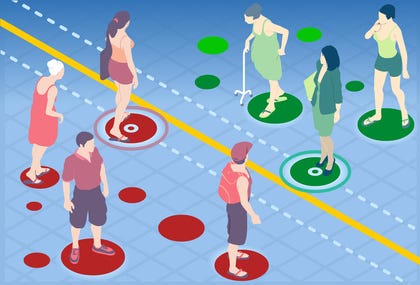
The two most commonly used techniques in unsupervised learning are principal component analysis (PCA) and clustering. PCA is one approach to learning what is called a latent variable model, and is a particular version of a blind signal separation technique. Other notable latent variable modeling approaches include expectation-maximization algorithm (EM) and Method of moments3.
PCA
PCA
produces a low-dimensional representation of a dataset by finding a
sequence of linear combinations of the variables that have maximal
variance, and are mutually uncorrelated. Another way to describe PCA is
that it is a transformation of possibly correlated variables into a set
of linearly uncorrelated variables known as principal components.
Each of the components
are mathematically determined and ordered by the amount of variability
or variance that each is able to explain from the data. Given that, the
first principal component accounts for the largest amount of variance,
the second principal component the next largest, and so on.
Each component is also orthogonal
to all others, which is just a fancy way of saying that they’re
perpendicular to each other. Think of the X and Y axis’ in a two
dimensional plot. Both axis are perpendicular to each other, and are
therefore orthogonal. While not
easy to visualize, think of having many principal components as being
many axis that are perpendicular to each other.
While
much of the above description of principal component analysis may be a
bit technical sounding, it is actually a relatively simple concept from a
high level. Think of having a bunch of data in any amount of
dimensions, although you may want to picture two or three dimensions for
ease of understanding.
Each
principal component can be thought of as an axis of an ellipse that is
being built (think cloud) to contain the data (aka fit to the data),
like a net catching butterflies. The first few principal components
should be able to explain (capture) most of the data, with the addition
of more principal components eventually leading to diminishing returns.
One
of the tricks of PCA is knowing how many components are needed to
summarize the data, which involves estimating when most of the variance
is explained by a given number of components. Another consideration is
that PCA is sensitive to feature scaling, which was discussed earlier in
this series.
PCA is also used for exploratory data analysis and data visualization.
Exploratory data analysis involves summarizing a dataset through
specific types of analysis, including data visualization, and is often
an initial step in analytics that leads to predictive modeling, data
mining, and so on.
Further
discussion of PCA and similar techniques is out of scope of this
series, but the reader is encouraged to refer to external sources for
more information.
Clustering
Clustering refers to a set of techniques and algorithms used to find clusters
(subgroups) in a dataset, and involves partitioning the data into
groups of similar observations. The concept of ‘similar observations’ is
a bit relative and subjective, but it essentially means that the data
points in a given group are more similar to each other than they are to
data points in a different group.
Similarity
between observations is a domain specific problem and must be addressed
accordingly. A clustering example involving the NFL’s Chicago Bears (go
Bears!) was given in chapter 1 of this series.
Clustering
is not a technique limited only to machine learning. It is a widely
used technique in data mining, statistical analysis, pattern
recognition, image analysis, and so on. Given the subjective and
unsupervised nature of clustering, often data preprocessing,
model/algorithm selection, and model tuning are the best tools to use to
achieve the desired results and/or solution to a problem.
There
are many types of clustering algorithms and models, which all use their
own technique of dividing the data into a certain number of groups of
similar data. Due to the significant difference in these approaches, the
results can be largely affected, and therefore one must understand
these different algorithms to some extent to choose the most applicable
approach to use.
K-means
and hierarchical clustering are two widely used unsupervised clustering
techniques. The difference is that for k-means, a predetermined number
of clusters (k) is used to partition the observations, whereas the
number of clusters in hierarchical clustering is not known in advance.
Hierarchical
clustering helps address the potential disadvantage of having to know
or pre-determine k in the case of k-means. There are two primary types
of hierarchical clustering, which include bottom-up and agglomerative.
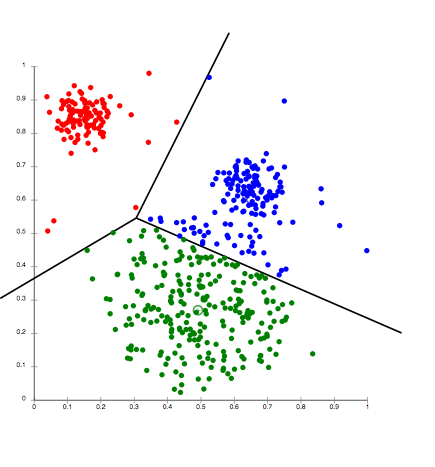
Here
is a visualization, courtesy of Wikipedia, of the results of running
the k-means clustering algorithm on a set of data with k equal to three.
Note the lines, which represent the boundaries between the groups of
data.
There are two types of clustering, which define the degree of grouping or containment of data. The first is called hard clustering, where every data point belongs to only one cluster and not the others. Soft clustering, or fuzzy clustering
on the other hand refers to the case where a data point belongs to a
cluster to a certain degree, or is assigned a likelihood (probability)
of belonging to a certain cluster.
Method comparison and general considerations
What
is the difference then between PCA and clustering? As mentioned, PCA
looks for a low-dimensional representation of the observations that
explains a good fraction of the variance, while clustering looks for
homogeneous subgroups among the observations.
An
interesting point to note is that in the absence of a target response,
there is no way to evaluate solution performance or errors as one does
in the supervised case. In other words, there is no objective way to
determine if you’ve found a solution. This is a significant
differentiator between supervised and unsupervised learning methods.
Predictive Analytics, Artificial Intelligence, and Data Mining, Oh My!
Machine
learning is often interchanged with terms like predictive analytics,
artificial intelligence, data mining, and so on. While machine learning
is certainly related to these fields, there are some notable
differences.
Predictive
analytics is a subcategory of a broader field known as analytics in
general. Analytics is usually broken into three sub-categories:
descriptive, predictive, and prescriptive.
Descriptive
analytics involves analytics applied to understanding and describing
data. Predictive analytics deals with modeling, and making predictions
or assigning classifications from data observations. Prescriptive
analytics deals with making data-driven, actionable recommendations or
decisions.
Artificial
intelligence (AI) is a super exciting field, and machine learning is
essentially a sub-field of AI due to the automated nature of the
learning algorithms involved. According to Wikipedia, AI has been
defined as the science and engineering of making intelligent machines, but also as the study and design of intelligent agents, where an intelligent agent is a system that perceives its environment and takes actions that maximize its chances of success
Statistical learning is becoming popularized due to Stanford’s related online course and its associated books: An Introduction to Statistical Learning, and The Elements of Statistical Learning.
Machine
learning arose as a subfield of artificial intelligence, statistical
learning arose as a subfield of statistics. Both fields are very
similar, overlap in many ways, and the distinction is becoming less
clear over time. They differ in that machine learning has a greater
emphasis on prediction accuracy and large scale applications, whereas
statistical learning emphasizes models and their related
interpretability, precision, and uncertainty.
Lastly,
data mining is a field that’s also often confused with machine
learning. Data mining leverages machine learning algorithms and
techniques, but also spans many other fields such as data science, AI,
statistics, and so on.
The
overall goal of the data mining process is to extract patterns and
knowledge from a data set, and transform it into an understandable
structure for further use. Data mining often deals with large amounts of
data, or big data.
Machine Learning in Practice
As
discussed throughout this series, machine learning can be used to
create predictive models, assign classifications, make recommendations,
and find patterns and insights in an unlabeled dataset. All of these
tasks can be done without requiring explicit programming.
Machine learning has been successfully used in the following non-exhaustive example applications1:
Spam filtering
Optical character recognition (OCR)
Search engines
Computer vision
Recommendation engines, such as those used by Netflix and Amazon
Classifying DNA sequences
Detecting fraud, e.g., credit card and internet
Medical diagnosis
Natural language processing
Speech and handwriting recognition
Economics and finance
Virtually anything else you can think of that involves data
In
order to apply machine learning to solve a given problem, the following
steps (or a variation) should to be taken, and should use machine
learning elements discussed throughout this series.
Define the problem to be solved and the project’s objective. Ask lots of questions along the way!
Determine the type of problem and type of solution required.
Collect and prepare the data.
Create,
validate, tune, test, assess, and improve your model and/or solution.
This process should be driven by a combination of technical (stats,
math, programming), domain, and business expertise.
Discover any other insights and patterns as applicable.
Deploy your solution for real-world use.
Report on and/or present results.
If
you encounter a situation where you or your company can benefit from a
machine learning-based solution, simply approach it using these steps
and see what you come up with. You may very well wind up with a super
powerful and scalable solution!
Summary
Congratulations to those that have read all five chapters in full! I would like to thank you very much for spending your precious time joining me on this machine learning adventure.
This
series took me a significant amount of time to write, so I hope that
this time has been translated into something useful for as many people
as possible.
At
this point, we have covered virtually all major aspects of the entire
machine learning process at a high level, and at times even went a
little deeper.
If
you were able to understand and retain the content in this series, then
you should have absolutely no problem participating in any conversation
involving machine learning and its applications. You may even have some
very good opinions and suggestions about different applications,
methods, and so on.
Despite
all of the information covered in this series, and the details that
were out of scope, machine learning and its related fields in practice
are also somewhat of an art. There are many decisions that need to be
made along the way, customized techniques to employ, as well as use
creative strategies in order to best solve a given problem.
A
high quality practitioner should also have a strong business acumen and
expert-level domain knowledge. Problems involving machine learning are
just as much about asking questions as they are about finding solutions.
If the question is wrong, then the solution will be as well.
Thank you again, and happy learning (with machines)!
We propose two efficient approximations to standard convolutional neural
networks: Binary-Weight-Networks and XNOR-Networks. In Binary-Weight-Networks,
the filters are approximated with binary values resulting in 32x memory saving.
In XNOR-Networks, both the filters and the input to convolutional layers are
binary. XNOR-Networks approximate convolutions using primarily binary
operations. This results in 58x faster convolutional operations and 32x memory
savings. XNOR-Nets offer the possibility of running state-of-the-art networks
on CPUs (rather than GPUs) in real-time. Our binary networks are simple,
accurate, efficient, and work on challenging visual tasks. We evaluate our
approach on the ImageNet classification task. The classification accuracy with
a Binary-Weight-Network version of AlexNet is only 2.9% less than the
full-precision AlexNet (in top-1 measure). We compare our method with recent
network binarization methods, BinaryConnect and BinaryNets, and outperform
these methods by large margins on ImageNet, more than 16% in top-1 accuracy.