https://medium.com/mlreview/modern-theory-of-deep-learning-why-does-it-works-so-well-9ee1f7fb2808
What can we learn from the latest research on the paradoxical effectiveness of Deep Learning “Alchemy”.
Motivation
Deep
Learning is currently being used for a variety of different
applications. But is frequently criticised for lacking a fundamental
theory that can fully answer why does it work so well. It’s only
recently that the winner of the Test-of-Time award at the Conference on
Neural Information Processing (NIPS) compared Deep Learning to Alchemy.
Although
Generalization Theory that explains why Deep Learning generalizes so
well is an open problem, in this article we would discuss most recent
theoretical and empirical advances in the field that attempt to explain
it.
The Paradox of Deep Learning
An
“apparent paradox” with Deep Learning is that it can generalize well in
practice despite its large capacity, numerical instability, sharp
minima, and nonrobustness.
In a recent paper “Understanding deep learning requires rethinking generalization”
it was shown that Deep Neural Networks (DNN) has enough capacity to
memorize ImageNet and CIFAR10 datasets with random labels. And it is
unclear why they find generalizable solutions on real data.
Another
important issue with deep architectures is numerical instabilities.
Numerical instabilities in derivative-based learning algorithms are
commonly called exploding or vanishing gradients.
Additional difficulties stem from instabilities of the underlying
forward model. That is the output of some networks can be unstable with
respect to small perturbations in the original features. In machine
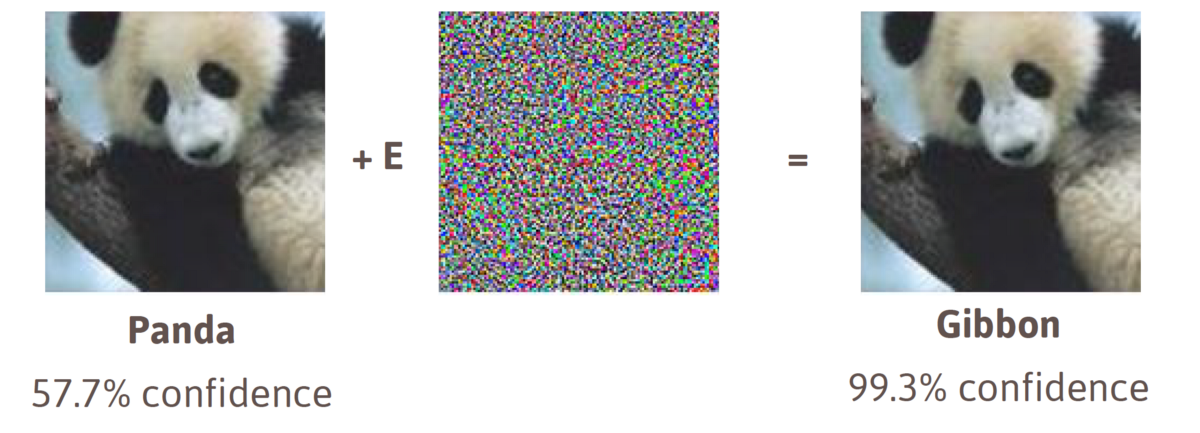
learning it is called non-robustness. An example of it is an adversarial attack illustrated in Figure 1.
Several
studies based their arguments for generalization in deep learning on
the flatness of minima of the loss function found by Stochastic Gradient
Descent (SGD). However, recently it was shown that “Sharp Minima Can Generalize For Deep Nets”
as well. More specifically, flat minima can be turned into sharp minima
via re-parameterization without changing the generalization.
Consequently, generalization can not be explained merely by the
robustness of parameter space only.
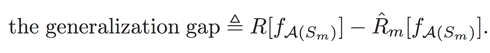
Generalization Theory
The
goal of generalization theory is to explain and justify why and how
improving accuracy on a training set improves accuracy on a test set.
The difference between these two accuracies is called generalization
error or “generalization gap”. More rigorously generalization gap can be
defined as a difference between the non-computable expected risk and
the computable empirical risk of a function f on a dataset Sm given a learning algorithm A:
Essentially if we bound the generalization gap with a small value it would guarantee that Deep Learning algorithm f generalizes
well in practice. Multiple theoretical bounds exist for generalization
gap based on model complexity, stability, robustness etc.
Two measures of model complexity are Rademacher complexity and Vapnik‑Chervonenkis (VC) dimension. Unfortunately, for the deep learning function f known bounds based on Radamacher complexity grow exponentially in depth of DNN. Which contradicts practical observation that deeper nets fit better to the training data and achieve smaller empirical errors.
Similarly, the generalization gap bound based on VC dimension grows
linearly in the number of trainable parameters and cannot account for
the practical observations with deep learning. In other words, these two
bounds are too conservative.
A much more useful approach was recently proposed by K Kawaguchi, LP Kaelbling, and Y Bengio.
Unlike others, they embrace the fact that usually deep learning models
are trained using train-validation paradigm. Instead of bounding the
non-computable expected risk with train error, they use validation
error. In this view, they propose the following intuition on why deep
learning generalizes well in practice: “we can generalize well because we can obtain a good model via model search with validation errors”. And prove the following bound for any δ > 0, with probability at least 1 − δ:
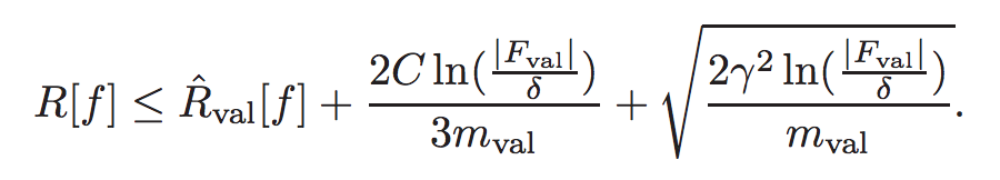
Importantly |Fval| is the number of times we use the validation dataset in our decision making to choose a final model, m is
the validation set size. This bound explains why deep learning had the
ability to generalize well, despite possible nonstability, nonrobustness
and sharp minimas. Somewhat an open question still remains why we are
able to find architectures and parameters that result in low validation
errors. Usually, architectures are inspired by real-world observations
and good parameters are searched using SGD that we would discuss next.
Stochastic Gradient Descent
SGD
is an inherent part of modern Deep Learning and apparently one of the
main reasons behind its generalization. So we would discuss its
generalization properties next.
In a recent paper “Data-Dependent Stability of Stochastic Gradient Descent” authors were able to prove that SGD is on-average stable algorithm under
some additional loss conditions. These conditions are fulfilled in
commonly used loss functions such as logistic/softmax losses in neural
nets with sigmoid activations. Stability, in this case, means how
sensitive is SGD to small perturbations in the training set. They take
it further to prove a data-dependant on-average bound for generalization
gap of SGD in non-convex functions such as deep neural nets:

where m is a training set size, T
number of training steps and γ characterizes how the curvature at the
initialization point affects stability. Which lead to at-least two
conclusions. First, the curvature of the objective function around the
initialization point has crucial influence. Starting from a point in a less curved region with low risk should yield higher stability, i.e faster generalization. In
practice it can be a good pre-screen strategy for picking good
initialization params. Second, considering the full pass, that is m = O(T), we simplify the bound to O(m⁻¹). That is the bigger training set, the smaller generalization gap.
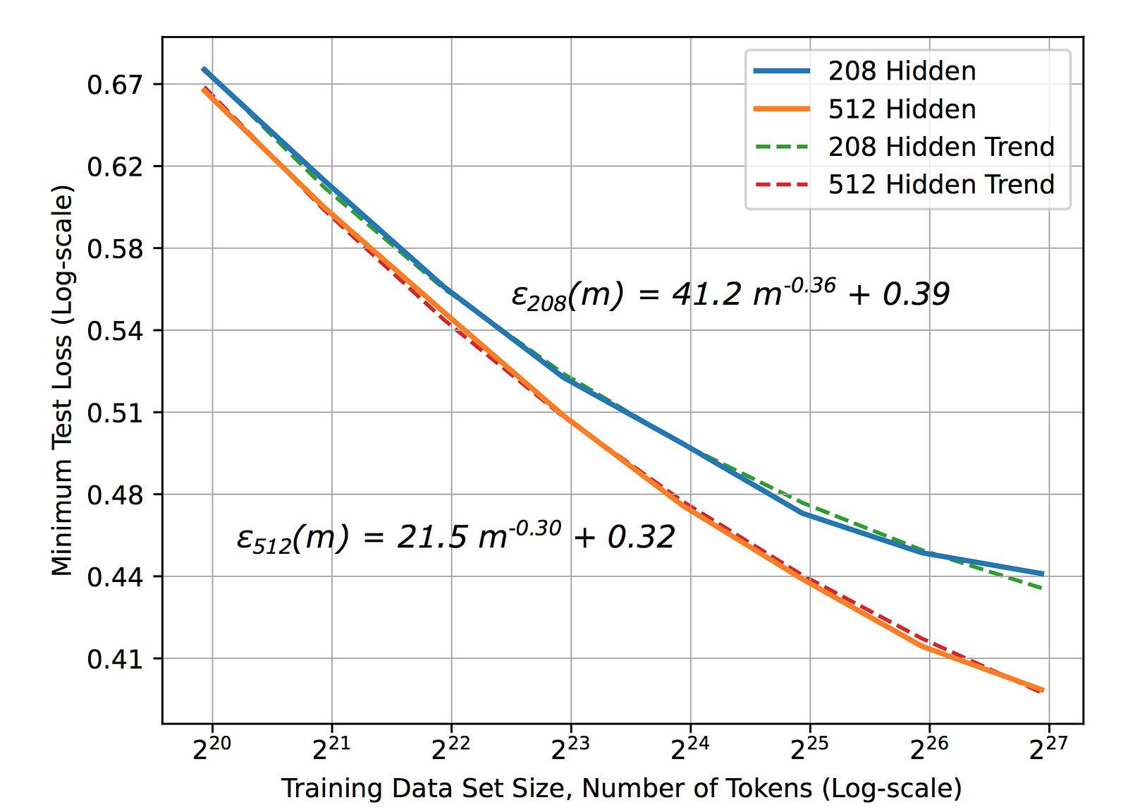
Interestingly,
there is a number of studies investigating learning curves. Most of
them show power-law generalization error, scaling as ε(m) ∼ mᵝ with exponent β = −0.5 or −1. Which is also aligned with the previously discussed paper. However, it’s important to mention the large-scale research by Baidu that was able to empirically observe this power-law (see Figure 2). However, the exponent β in real applications was between−0.07 and −0.35. Which has to be still explained by theory.
Additionally,
there is both theoretical and empirical evidence of batch size effect
on generalization of SGD. Intuitively a small batch training introduces
noise to the gradients, and this noise drives the SGD away from sharp
minima, thus enhancing generalization. In a recent paper from Google it was shown that the optimum batch size is proportional to the learning rate and the training set size. Or simply put in other words, “Don’t Decay the Learning Rate, Increase the Batch Size”. Similarly scaling rules were derived for SGD with momentum: Bopt ~1/(1 − m), where Bopt is an optimal batch size and m is momentum. Alternatively, all conclusions can be summarised by the following equation:

where 𝜖 is learning rate, N is training set size, m is momentum and B is batch size.
Conclusions
In
the last few years, there has been an increasingly growing interest in
the fundamental theory behind the paradoxical effectiveness of Deep
Learning. And although there are still open research problems, modern
Deep Learning by any means is far from being called Alchemy. In this
article we discussed the generalization perspective on the problem which
leads us to a number of practical conclusions:
- Select initialization params in a less curved region and lower risk. Curvature can be efficiently estimated by Hessian-vector multiplication method.
- Rescale the batch size, when changing momentum.
- Don’t decay the learning rate, increase the batch size.
No comments:
Post a Comment