A 'Brief' History of Neural Nets and Deep Learning, Part 2

http://www.andreykurenkov.com/writing/a-brief-history-of-neural-nets-and-deep-learning-part-2/

This is the second part of ‘A Brief History of Neural Nets and Deep Learning’. Part 1 is here, and Parts 3 and 4 are here and here. In this part, we will look into several strains of research that made rapid progress following the development of backpropagation and until the late 90s, which we shall see later are the essential foundations of Deep Learning.

Neural Nets Gain Vision

Yann LeCun's LeNet demonstrated.

With the secret to training multilayer neural nets uncovered, the topic was once again ember-hot and the lofty ambitions of Rosenblatt seemed to perhaps be in reach. It took only until 1989 for another key finding now universally cited in textbooks and lectures to be published

: “Multilayer feedforward networks are universal approximators”. Essentially, it mathematically proved that multiple layers allow neural nets to theoretically implement any function, and certainly XOR.
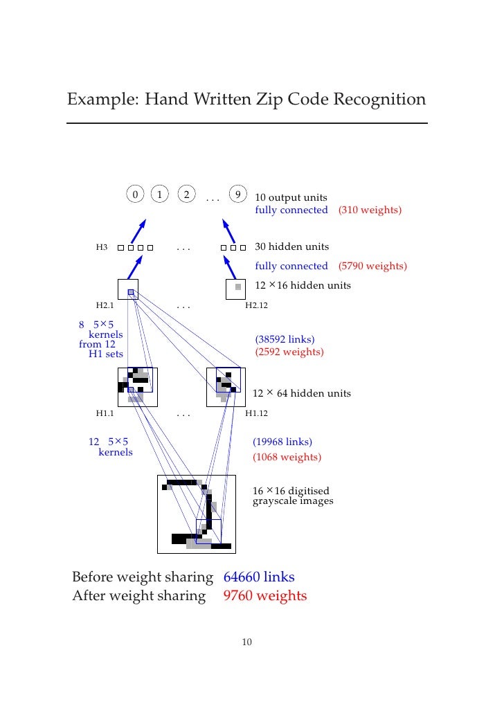
But, this is mathematics, where you could imagine having endless memory and computation power should it be needed - did backpropagation allow neural nets to be used for anything in the real world? Oh yes. Also in 1989, Yann LeCunn et al. at the AT&T Bell Labs demonstrated a very significant real-world application of backpropagation in "”Backpropagation Applied to Handwritten Zip Code Recognition”

. You may think it fairly unimpressive for a computer to be able to correctly understand handwritten digits, and nowdays it is indeed quite quaint, but prior to the publication the messy and inconsistent scrawls of us humans proved a major challenge to the much more tidy minds of computers. The publication, working with a large dataset from the US Postal Service, showed neural nets were entirely capable of this task. And much more importantly, it was first to highlight the practical need for a key modifications of neural nets beyond plain backpropagation toward modern deep learning:

“Classical work in visual pattern recognition has demonstrated the advantage of extracting local features and combining them to form higher order features. Such knowledge can be easily built into the network by forcing the hidden units to combine only local sources of information. Distinctive features of an object can appear at various location on the input image. Therefore it seems judicious to have a set of feature detectors that can detect a particular instance of a feature anywhere on the input place. Since the precise location of a feature is not relevant to the classification, we can afford to lose some position information in the process. Nevertheless, approximate position information must be preserved, to allow the next levels to detect higher order, more complex features (Fukushima 1980; Mozer 1987).”

A visualization of how this neural net works. (Source)

Or, more concretely: the first hidden layer of the neural net was convolutional - instead of having each neuron have a different weight for each pixel of the input image (40x60=2400 weights), the neurons only had a small set of weights (5x5=25) that were applied a whole bunch of small subsets of the image of the same size. So, for instance instead of having 4 different neurons learn to detect 45 degree lines in each of the 4 corners of the input image, a single neuron could learn to detect 45 degree lines on subsets of the image and do that everywhere within it. Layers past the first work in a similar way, but take in the ‘local’ features locations found in the previous hidden layer rather than pixel images, and so ‘see’ successively larger portions of the image since they are combining information about increasingly larger subsets of the image. Finally, the last two layers are just plain normal neural net layers that use the higher-order larger features generated by the convolutional layers to determine which digit the input image corresponds to. The method proposed in this 1989 paper went on to be the basis of nationally deployed check-reading systems, as demonstrated by LeCun in this gem of a video:

The reason for why this is helpful is intuitively if not mathematically clear: without such constraints the network would have to learn the same simple things (such as detecting 45 degree lines, small circles, etc) a whole bunch of times for each portion of the image. But with the constraint there, only one neuron would need to learn each simple feature - and with far fewer weights overall, it could do so much faster! Moreover, since the pixel-exact location of such features does not matter it could basically skip neighboring subsets of the image - subsampling, now known as a type of pooling - when applying the weights, further reducing the training time. The addition of these two types of layers - convolutional and pooling layers - are the primary distinctions of Convolutional Neural Nets (CNNs/ConvNets) from plain old neural nets.

A nice visualization of CNN operation (Source)

At that time, the convolution idea was called ‘weight sharing’, and it was actually discussed in the 1986 extended analysis of backpropagation by Rumelhart, Hinton, and Williams

. Remarkably, Minsky and Papert’s 1969 analysis of Perceptrons was thorough enough to pose a problem that motivated this idea. But, as before, others have also independently explored the concept - namely, Kunihiko Fukushima in 1980 with his notion of the Neurocognitron

. And, as before, the ideas behind it drew inspiration from studies of the brain:

“According to the hierarchy model by Hubel and Wiesel, the neural network in the visual cortex has a hierarchy structure: LGB (lateral geniculate body)->simple cells->complex cells->lower order hypercomplex cells->higher order hypercomplex cells. It is also suggested that the neural network between lower order hypercomplex cells and higher order hypercomplex cells has a structure similar to the network between simple cells and complex cells. In this hierarchy, a cell in a higher stage generally has a tendency to respond selectively to a more complicated feature of the stimulus pattern, and, at the same time, has a larger receptive field, and is more insensitive to the shift in position of the stimulus pattern. … Hence, a structure similar to the hierarchy model is introduced in our model.”

LeCun continued to be a major proponent of CNNs at Bell Labs, and his work on them resulted in major commercial use for check-reading in the mid 90s - his talks and interviews often include the fact that “At some point in the late 1990s, one of these systems was reading 10 to 20% of all the checks in the US.”

.

Neural Nets Go Unsupervised

Automating the rote and utterly uninteresting task of reading checks is a great instance of what Machine Learning can be used for. Perhaps a less predictable application? Compression. Meaning, of course, finding a smaller representation of some data from which the original data can be reconstructed. Learned compression may very well outperform stock compression schemes, in the case the learning algorithm can find features within the data stock methods would miss. And it is very easy to do - just train a neural net with a small hidden layer to just output the input:

An autoencoder neural net. (Source)

This is an autoencoder neural net, and is a method for learning compression - efficiently translating (encoding) data to a compact format and back to itself (auto). See, the output layer computes its outputs, which ideally are the same as the input to the neural net, using only the hidden layer’s outputs. Since the hidden layer has fewer outputs than does the input layer, the output of the hidden layer is the compressed representation of the input data, which can be reconstructed with the output layer.

A more explicit view of an autoencoder compression. (Source)

Notice a neat thing here: the only thing we need for training is some input data. This is in contrast to the requirement of supervised machine learning, which needs a training set of input-output pairs (labeled data) in order to approximate a function that generalizes can compute such outputs from such inputs. And indeed, autoencoders are not a form of supervised learning; they are a form of unsupervised learning, which only needs a set of input data (unlabeled data) in order to find some hidden structure within that data. In other words, unsupervised learning does not approximate a function so much as it derives one from the input data to another useful representation of that data. In this case, this representation is just a smaller one from which the original data can still be reconstructed, but it can also be used for finding groups of similar data (clustering) or other inference of latent variables (some aspect that is known to exist for the data but the value of which is not known).

Clustering, a very common unsupervised learning application. (Source)

There were other unsupervised applications of neural networks explored prior to and after the discovery of backpropagation, most notably Self Organizing Maps

, which produce a low-dimensional representation of data good for visualization, and Adapative Resonance Theory

, which can learn to classify arbitrary input data without being told correct classifications. If you think about it, it is intuitive that quite a lot can be learned from unlabeled data. Say you have a dataset of a bunch of images of handwritten digits, without labels of which digit each image corresponds to. Well, an image with some digit in that dataset most likely looks most like all the other images with that same digit, and so though a computer may not know which digit all those images correspond to, it should still be able to find that they all correspond to the same one. This, pattern recognition, is really what most of machine learning is all about, and arguably also is the basis for the great powers of the human brain. But, let us not digress from our exciting deep learning journey, and get back to autoencoders.

Self Organizing Maps - mapping a large vector of inputs into a grid of neuron outputs, where each output is a cluster. Nearby neurons represent similar clusters. (Source)

As with weight-sharing, the idea of autoencoders was first discussed in the aforementioned extensive 1986 analysis of backpropagation ³, and as with weight-sharing it resurfaced in more research in the following years

, including by Hinton himself

. This paper, with the fun title “Autoencoders, Minimum Description Length, and Helmholts Free Energy”, posits that “A natural approach to unsupervised learning is to use a model that defines probability distribution over observable vectors” and uses a neural net to learn such a model. So here’s another neat thing you can do with neural nets: approximate probability distributions.

Neural Nets Gain Beliefs

In fact, before being co-author of the seminal 1986 paper on backpropagation learning algorithm, Hinton worked on a neural-net approach for learning probability distributions in the 1985 “A Learning Algorithm for Boltzmann Machines”

. Boltzmann Machines are networks just like neural nets and have units that are very similar to Perceptrons, but instead of computing an output based on inputs and weights, each unit in the network can compute a probability of it having a value of 1 or 0 given the values of connected units and weights. The units are therefore stochastic - they behave according to a probability distribution, rather than in a known deterministic way. The Boltzmann part refers to a probability distribution that has to do with the states of particles in a system based the particles’ energy and on the thermodynamic temperature of that system. This distribution defines not only the mathematics of the Boltzmann machines, but also the interpretation - the units in the network themselves have energies and states, and learning is done by minimizing the energy of the system and with direct inspirartion from thermodynamics. Though a bit unintuitive, this energy-based interpretation is actually just one example of an energy-based model, and fits in the energy-based learning theoretical framework with which many learning algorithms can be expressed

.

That there is a common theoretical framework for a bunch of learning methods is not too surprising, since at the end of the day all of learning boils down to optimization. Quoting from the above cited tutorial:

"Training an EBM consists in finding an energy function that produces the best Y for any X ... The architecture of the EBM is the internal structure of the parameterized energy function E(W, Y, X) ... This quality measure is called the loss functional (i.e. a function of function) and denoted L(E,S). ... In order to find the best energy function [] we need a way to assess the quality of any particular energy function, based solely on two elements: the training set, and our prior knowledge about the task. For simplicity, we often denote it L(W,S) and simply call it the loss function. The learning problem is simply to find the W that minimizes the loss."

So, the key to energy based models is recognizing all these algorithms are essentially different ways to optimize a pair of functions, that can be called the energy function E and loss function L, by finding a set of good values to a bunch of variables that can be denoted W using data denoted X for input and Y for the output. It's really a very broad definition for a framework, but still nicely encapsulates what a lot of algorithms fundamentally do.

A simple belief, or bayesian, network - a Boltzmann machine is basically this but with undirected/symmetric connections and trainable weights to learn the probabilities in a particular fashion. (Source)

Back to Boltzmann Machines. When such units are put together into a network, they form a graph, and so are a graphical model of data. Essentially, they can do something very similar to normal neural nets: some hidden units compute the probability of some hidden variables (the outputs - classifications or features for data) given known values of visible units that represent visible variables (the inputs - pixels of images, characters in text, etc.). In the nice known example of classifying images of digits, the hidden variables are the actual digit values, and the visible variables are the pixels of the image; given an image of the digit ‘1’ as input, the value of visible units is known and the hidden unit modeling the probability of the image representing a ‘1’ should have a high output probability.

An example Boltzmann machine. Each line has an associated weight, as with a neural net. Notice there are no layers here - everything can sort of be connected to everything. We'll talk about this variation on neural net in a little bit... (Source)

So, for the classification task, there is now a nice way of computing the probability of each category. This is very analogous to actually computing the output values of a normal classification neural net, but these nets have another neat trick: they can generate plausible looking input data. This follows from the probability equations involved - not only does the net learn the probabilities of values for the hidden variables given known values for the visible variables, but it also the inverse of that - visible probabilities given known hidden values. So, if we want to generate a ‘1’ digit image, the units corresponding to the pixel variables have known probabilities of outputting a 1 and an image can be probabilistically generated - these networks are generative graphical models. Though it is possible to do supervised learning with very similar goals as normal neural nets, the unsupervised learning task of learning a good generative model - probabilistically learning the hidden structure of some data - is commonly what these nets are used for. Most of this was not really that novel, but the learning algorithm presented and the particular formulation that enabled it were, as stated in the paper itself:

“Perhaps the most interesting aspect of the Boltzmann Machine formulation is that it leads to a domain-independent learning algorithm that modifies the connection strengths between units in such a way that the whole network develops an internal model which captures the underlying structure of its environment. There has been a long history of failure in the search for such algorithms (Newell, 1982), and many people (particularly in Artificial Intelligence) now believe that no such algorithms exist.”

Having learned the classical neural net models first, it took me a while to understand the notion behind these probabilistic nets. To elaborate, let me present a quote from the paper itself that restates all that I have said above quite well:

"The network modifies the strengths of its connections so as to construct an internal generative model that produces examples with the same probability distribution as the examples it is shown. Then, when shown any particular example, the network can “interpret” it by finding values of the variables in the internal model that would generate the example.
...
The machine is composed of primitive computing elements called units that are connected to each other by bidirectional links. A unit is always in one of two states, on or off, and it adopts these states as a probabilistic function of the states of its neighboring units and the weights on its links to them. The weights can take on real values of either sign. A unit being on or off is taken to mean that the system currently accepts or rejects some elemental hypothesis about the domain. The weight on a link represents a weak pairwise constraint between two hypotheses. A positive weight indicates that the two hypotheses tend to support one another; if one is currently accepted, accepting the other should be more likely. Conversely, a negative weight suggests, other things being equal, that the two hypotheses should not both be accepted. Link weights are symmetric, having the same strength in both directions (Hinton & Sejnowski, 1983)."

Without delving into the full details of the algorithm, here are some highlights: it is a variant on maximum-likelihood algorithms, which simply means that it seeks to maximize the probability of the net’s visible unit values matching with their known correct values. Computing the actual most likely value for each unit turns all at the same time out to be much too computationally expensive, so in training Gibbs Sampling - starting the net with random unit values and iteratively reassigning values to units given their connections’ values - is used to give some actual known values. When learning using a training set, the visible units are just set to have the value of the current training example, so sampling is done to get values for the hidden units. Once some ‘real’ values are sampled, we can do something similar to backpropagation - take a derivative for each weight to see how we can change so as to increase the probability of the net doing the right thing.
As with neural net, the algorithm can be done both in a supervised fashion (with known values for the hidden units) or in an unsupervised fashion. Though the algorithm was demonstrated to work (notably, with the same ‘encoding’ problem that autoencoder neural nets solve), it was soon apparent that it just did not work very well - Redford M. Neal’s 1992 “Connectionist learning of belief networks”

justified a need for a faster approach by stating that: “These capabilities would make the Boltzmann machine attractive in many applications, were it not that its learning procedure is generally seen as being painfully slow”. And so Neal introduced a similar idea in the belief net, which is essentially like a Boltzmann machine with directed, forward connections (so that there are again layers, as with the the neural nets we have seen before, and unlike the Boltzmann machine image above). Without getting into mucky probability math, this change allowed the nets to be trained with a faster learning algorithm. We actually saw a ‘belief net’ just above with the sprinkler and rain variables, and the term was chosen precisely because this sort of probability-based modeling has a close relationship to idea from the mathematical field of probability, in addition to its link to the field of Machine Learning.

An explanation of belief nets. (Source)

Though this approach was an advance upon Boltzmann machines, it was still just too slow - the math for correctly deriving probabilistic relations between variables is such that a ton of computation is typically required without some simplifying tricks. And so Hinton, along with Neal and two other co-authors, soon came up with extra tricks in the 1995 “The wake-sleep algorithm for unsupervised neural networks”

. These tricks were such that they once again such that they called for a slightly different belief net setup, which was now deemed “The Helmholtz Machine”

. Skirting the details once again, the key idea was to have separate sets of weights for inferring hidden variables from visible variables (recognition weights) and for vice versa (generative weights), and to keep the directed aspect of Neal’s belief nets. This allows the training to be done much faster, while being applicable to the same unsupervised and supervised learning problems of Boltzmann Machines.

When Hinton talks of the Wake Sleep algorithm, he often notes how gross the simplifying assumption being made is, and that despite that the algorithm just works. Again I will quote as the paper itself explains the assumption well:

"The key simplifying assumption is that the recognition distribution for a particular example d, Q is factorial (separable) in each layer. If there are h stochastic binary units in a layer B, the portion of the distribution P(B,d) due to that layer is determined by 2^(h - 1) probabilities. However, Q makes the assumption that the actual activity of any one unit in layer P is independent of the activities of all the other units in that layer, given the activities of all the units in the lower layer, l - 1, so the recognition model needs only specify h probabilities rather than 2" - 1. The independence assumption allows F(d; 8.4) to be evaluated efficiently, but this computational tractability is bought at a price, since the true posterior is unlikely to be factorial
...
The generative model is taken to be factorial in the same way, although one should note that factorial generative models rarely have recognition distributions that are themselves exactly factorial."

Note the Neal's belief nets also implicitly made the probabilities factorize by having layers of units with only forward-facing directed connections.

Finally, belief nets could be trained somewhat fast! Though not quite as influential, this algorithmic advance was a significant enough forward step for unsupervised training of belief nets that it could be seen as a companion to the now almost decade-old breakthrough that was backpropagation. But, by this point new machine learning methods had begun to also emerge, and people were again beginning to be skeptical of neural nets since so much of their ideas seemed intuition-based and since computers were still barely able to meet their computational needs. As we’ll see in part 3, a new AI Winter for neural nets began just a few years later…

1. Kurt Hornik, Maxwell Stinchcombe, Halbert White, Multilayer feedforward networks are universal approximators, Neural Networks, Volume 2, Issue 5, 1989, Pages 359-366, ISSN 0893-6080, http://dx.doi.org/10.1016/0893-6080(89)90020-8. ↩
   
2. LeCun, Y; Boser, B; Denker, J; Henderson, D; Howard, R; Hubbard, W; Jackel, L, “Backpropagation Applied to Handwritten Zip Code Recognition,” in Neural Computation , vol.1, no.4, pp.541-551, Dec. 1989 89 ↩
   
3. D. E. Rumelhart, G. E. Hinton, and R. J. Williams. 1986. Learning internal representations by error propagation. In Parallel distributed processing: explorations in the microstructure of cognition, vol. 1, David E. Rumelhart, James L. McClelland, and CORPORATE PDP Research Group (Eds.). MIT Press, Cambridge, MA, USA 318-362 ↩ ↩²
   
4. Fukushima, K. (1980), ‘Neocognitron: A Self-Organizing Neural Network Model for a Mechanism of Pattern Recognition Unaffected by Shift in Position’, Biological Cybernetics 36 , 193–202 . ↩
   
5. Gregory Piatetsky, ‘KDnuggets Exclusive: Interview with Yann LeCun, Deep Learning Expert, Director of Facebook AI Lab’ Feb 20, 2014. http://www.kdnuggets.com/2014/02/exclusive-yann-lecun-deep-learning-facebook-ai-lab.html ↩
   
6. Teuvo Kohonen. 1988. Self-organized formation of topologically correct feature maps. In Neurocomputing: foundations of research, James A. Anderson and Edward Rosenfeld (Eds.). MIT Press, Cambridge, MA, USA 509-521. ↩
   
7. Gail A. Carpenter and Stephen Grossberg. 1988. The ART of Adaptive Pattern Recognition by a Self-Organizing Neural Network. Computer 21, 3 (March 1988), 77-88. ↩
   
8. H. Bourlard and Y. Kamp. 1988. Auto-association by multilayer perceptrons and singular value decomposition. Biol. Cybern. 59, 4-5 (September 1988), 291-294. ↩
   
9. P. Baldi and K. Hornik. 1989. Neural networks and principal component analysis: learning from examples without local minima. Neural Netw. 2, 1 (January 1989), 53-58. ↩
   
10. Hinton, G. E. & Zemel, R. S. (1993), Autoencoders, Minimum Description Length and Helmholtz Free Energy., in Jack D. Cowan; Gerald Tesauro & Joshua Alspector, ed., ‘NIPS’ , Morgan Kaufmann, , pp. 3-10 . ↩
    
11. Ackley, D. H., Hinton, G. E., & Sejnowski, T. J. (1985). A learning algorithm for boltzmann machines*. Cognitive science, 9(1), 147-169. ↩
    
12. LeCun, Y., Chopra, S., Hadsell, R., Ranzato, M., & Huang, F. (2006). A tutorial on energy-based learning. Predicting structured data, 1, 0. ↩
    
13. Neal, R. M. (1992). Connectionist learning of belief networks. Artificial intelligence, 56(1), 71-113. ↩
    
14. Hinton, G. E., Dayan, P., Frey, B. J., & Neal, R. M. (1995). The” wake-sleep” algorithm for unsupervised neural networks. Science, 268(5214), 1158-1161. ↩
    
15. Dayan, P., Hinton, G. E., Neal, R. M., & Zemel, R. S. (1995). The helmholtz machine. Neural computation, 7(5), 889-904. ↩