Background
Backpropagation is a common method for training a neural network. There is no shortage of papers online that attempt to explain how backpropagation works, but few that include an example with actual numbers. This post is my attempt to explain how it works with a concrete example that folks can compare their own calculations to in order to ensure they understand backpropagation correctly.If this kind of thing interests you, you should sign up for my newsletter where I post about AI-related projects that I’m working on.
Backpropagation in Python
You can play around with a Python script that I wrote that implements the backpropagation algorithm in this Github repo.Overview
For this tutorial, we’re going to use a neural network with two inputs, two hidden neurons, two output neurons. Additionally, the hidden and output neurons will include a bias.Here’s the basic structure:

In order to have some numbers to work with, here’s are the initial weights, the biases, and training inputs/outputs:
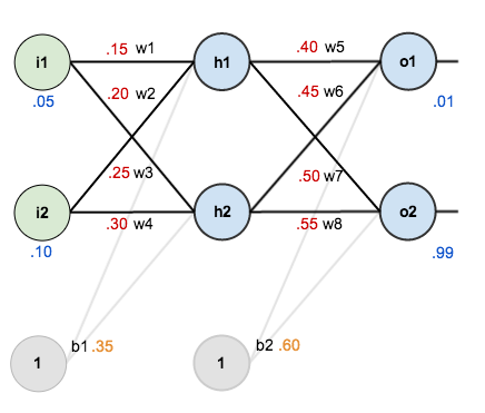
The goal of backpropagation is to optimize the weights so that the neural network can learn how to correctly map arbitrary inputs to outputs.
For the rest of this tutorial we’re going to work with a single training set: given inputs 0.05 and 0.10, we want the neural network to output 0.01 and 0.99.
The Forward Pass
To begin, lets see what the neural network currently predicts given the weights and biases above and inputs of 0.05 and 0.10. To do this we’ll feed those inputs forward though the network.We figure out the total net input to each hidden layer neuron, squash the total net input using an activation function (here we use the logistic function), then repeat the process with the output layer neurons.
Total net input is also referred to as just net input by some sources.
Here’s how we calculate the total net input for  :
:

We then squash it using the logistic function to get the output of
:
Carrying out the same process for
 we get:
We repeat this process for the output layer neurons, using the output from the hidden layer neurons as inputs.
Here’s the output for
 :
:


And carrying out the same process for
 we get:
Calculating the Total Error
We can now calculate the error for each output neuron using the squared error function and sum them to get the total error:^{2}")
Some sources refer to the target as the ideal and the output as the actual.
The  is included so that exponent is cancelled when we differentiate later
on. The result is eventually multiplied by a learning rate anyway so it
doesn’t matter that we introduce a constant here [1].
is included so that exponent is cancelled when we differentiate later
on. The result is eventually multiplied by a learning rate anyway so it
doesn’t matter that we introduce a constant here [1].
For example, the target output for
is included so that exponent is cancelled when we differentiate later
on. The result is eventually multiplied by a learning rate anyway so it
doesn’t matter that we introduce a constant here [1]. is 0.01 but the neural network output 0.75136507, therefore its error is:^{2} = \frac{1}{2}(0.01 - 0.75136507)^{2} = 0.274811083")
Repeating this process for
we get:
The total error for the neural network is the sum of these errors:

The Backwards Pass
Our goal with backpropagation is to update each of the weights in the network so that they cause the actual output to be closer the target output, thereby minimizing the error for each output neuron and the network as a whole.Output Layer
Consider . We want to know how much a change in affects the total error, aka
  .
. is read as “the partial derivative of
  with respect to
  “. You can also say “the gradient with respect to “.
Visually, here’s what we’re doing:

We need to figure out each piece in this equation.
First, how much does the total error change with respect to the output?
^{2} + \frac{1}{2}(target_{o2} - out_{o2})^{2}")
^{2 - 1} * -1 + 0")
 = -(0.01 - 0.75136507) = 0.74136507")
") is sometimes expressed as
is sometimes expressed as 
When we take the partial derivative of the total error with respect to  , the quantity
 ^{2}") becomes zero because does not affect it which means we’re taking the derivative of a constant which is zero.
becomes zero because does not affect it which means we’re taking the derivative of a constant which is zero.
Next, how much does the output of , the quantity becomes zero because does not affect it which means we’re taking the derivative of a constant which is zero. change with respect to its total net input?The partial derivative of the logistic function is the output multiplied by 1 minus the output:

 = 0.75136507(1 - 0.75136507) = 0.186815602")
Finally, how much does the total net input of
 change with respect to ?
} + 0 + 0 = out_{h1} = 0.593269992")
Putting it all together:


You’ll often see this calculation combined in the form of the delta rule:
 * out_{o1}(1 - out_{o1}) * out_{h1}")
Alternatively, we have and
and  which can be written as
  , aka
, aka  (the Greek letter delta) aka the node delta. We can use this to rewrite the calculation above:

 * out_{o1}(1 - out_{o1})")
Therefore:

Some sources extract the negative sign from so it would be written as:

To decrease the error, we then subtract this value from the current
weight (optionally multiplied by some learning rate, eta, which we’ll
set to 0.5):Alternatively, we have
and which can be written as , aka (the Greek letter delta) aka the node delta. We can use this to rewrite the calculation above:Therefore:
Some sources extract the negative sign from
so it would be written as:
Some sources use  (alpha) to represent the learning rate, others use
  (eta), and others even use
  (epsilon).
We can repeat this process to get the new weights (alpha) to represent the learning rate, others use (eta), and others even use (epsilon). ,
,  , and
, and  :
:


We perform the actual updates in the neural network after we have the new weights leading into the hidden layer neurons (ie, we use the original weights, not the updated weights, when we continue the backpropagation algorithm below).
Hidden Layer
Next, we’ll continue the backwards pass by calculating new values for ,
,  ,
,  , and
, and  .
.Big picture, here’s what we need to figure out:

Visually:

We’re going to use a similar process as we did for the output layer, but slightly different to account for the fact that the output of each hidden layer neuron contributes to the output (and therefore error) of multiple output neurons. We know that
 affects both
  and
and  therefore the
  needs to take into consideration its effect on the both output neurons:
Starting with
 :
:
We can calculate
 using values we calculated earlier:
And
 is equal to :
Plugging them in:

Following the same process for
 , we get:
Therefore:

Now that we have
, we need to figure out  and then
  for each weight:
 = 0.59326999(1 - 0.59326999 ) = 0.241300709")
We calculate the partial derivative of the total net input to
with respect to the same as we did for the output neuron:
Putting it all together:

You might also see this written as:
 * \frac{\partial out_{h1}}{\partial net_{h1}} * \frac{\partial net_{h1}}{\partial w_{1}}")
 * out_{h1}(1 - out_{h1}) * i_{1}")

We can now update :
Repeating this for
, , and 


Finally, we’ve updated all of our weights! When we fed forward the 0.05 and 0.1 inputs originally, the error on the network was 0.298371109. After this first round of backpropagation, the total error is now down to 0.291027924. It might not seem like much, but after repeating this process 10,000 times, for example, the error plummets to 0.000035085. At this point, when we feed forward 0.05 and 0.1, the two outputs neurons generate 0.015912196 (vs 0.01 actual) and 0.984065734 (vs 0.99 actual).
If you’ve made it this far and found any errors in any of the above or can think of any ways to make it clearer for future readers, don’t hesitate to drop me a note. Thanks!
No comments:
Post a Comment