Today, we are announcing the open source release of DeepLab2, a modern TensorFlow library for deep labeling that aims to facilitate future research on dense pixel labeling by providing a unified, state-of-the-art, and easy-to-use TensorFlow codebase → https://goo.gle/3d3SnVE
To
climb the AI ladder with supervised learning may require “teaching” the
computer all the concepts that matter to us by showing tons of examples
where these concepts occur. This is not how humans learn: yes, thanks
to language we get some examples illustrating new named concepts that
are given to us, but the bulk of what we observe does not come labeled,
at least initially.
His reply makes a lot of sense both from a neuroscientific perspective and a practical perspective.Labeling data is expensive in terms of time as well as money. The obvious solution to this problem is to figure out a way to either:
(a) Make ML algorithms work without labeled data (i.e. Unsupervised Learning)
(b) Automatically label data or use large amounts of unlabeled data along with small amounts of labeled data (i.e. Semi-Supervised Learning)
Unsupervised learning is quite a difficult problem to solve, as Yann LeCun mentions in this article:
“We know the ultimate answer is unsupervised learning, but we don’t have the answer yet.”
However,
of late there has been renewed interest in Semi-Supervised Learning
which is reflected in both academic and industrial research. Here’s a
graph showing the number of research papers related to Semi-Supervised
Learning on Google Scholar by year.
Semi-Supervised Learning Research Papers by Year
In
this blog, we’ll take an in-depth look at Pseudo-Labeling — a simple
Semi-Supervised Learning (SSL) algorithm. Although Pseudo-Labeling is a
naive approach, it gives us an excellent opportunity to understand the
challenges with SSL and provides a foundation to learn some of the
modern improvements like MixMatch, Virtual Adversarial Training, etc.
Outline:
What is Pseudo-Labeling?
Understanding the Pseudo-Labeling method
Implementing Pseudo-Labeling
Why does Pseudo-Labeling work?
When does Pseudo-Labeling not work well?
Pseudo-Labeling with conventional ML algorithms
Challenges with Semi-Supervised Learning
1. What is Pseudo-Labeling?
First proposed by Lee in 2013 [1],
the pseudo-labeling method uses a small set of labeled data along with a
large amount of unlabeled data to improve a model’s performance. The
technique itself is incredibly simple and follows just 4 basic steps:
Train model on a batch of labeled data
Use the trained model to predict labels on a batch of unlabeled data
Use the predicted labels to calculate the loss on unlabeled data
Combine labeled loss with unlabeled loss and backpropagate
…and repeat.
This technique might seem quite strange — almost similar to the hundreds of “free energy device” videos on youtube. However, Pseudo-Labeling has been successfully used on several problems. In fact, in a Kaggle competition, a team used Pseudo-Labeling to improve their model’s performance just enough to secure the 1st place and win $25,000.
We’ll take a look at why this works in a bit, for now, let’s look at some details.
2. Understanding the Pseudo-Labeling method
Pseudo-labeling
trains the network with labeled and unlabeled data simultaneously in
each batch. This means for each batch of labeled and unlabeled data, the
training loop does:
One single forward pass on the labeled batch to calculate the loss → This is the labeled loss
One forward pass on the unlabeled batch to predict the “pseudo labels” for the unlabeled batch
Use this “pseudo label” to calculate the unlabeled loss.
Now
instead of simply adding the unlabeled loss with the labeled loss, Lee
proposes using weights. The overall loss function looks like this:
Equation [15] Lee (2013) [1]
Or in simpler words:
In
the equation, the weight (alpha) is used to control the contribution of
unlabeled data to the overall loss. In addition, the weight is a
function of time (epochs) and is slowly increased during training. This
allows the model to focus more on the labeled data initially when the
performance of the classifier can be bad. As the model’s performance
increases over time (epochs), the weight increases and the unlabeled
loss has more emphasis on the overall loss.
Lee proposes using the following equation for alpha (t) :
Equation [16] Lee (2013) [1]
where alpha_f = 3, T1 = 100 and T2 = 600. All of these are hyperparameters that change based on the model and the dataset.
Let’s check how Alpha changes with the epochs:
Variation of Alpha with Epochs
In
the first T1 epochs (100 in this case) the weight is 0 — effectively
forcing the model to train only on the labeled data. After T1 epochs,
the weight linearly increases to alpha_f (3 in this case) until T2
epochs (600 in this case) — this allows the model to slowly incorporate
the unlabeled data. T2 and alpha_f control the rate at which the weight
increases and the value after saturation respectively.
If you’re familiar with optimization theory you might recognize this equation from Simulated Annealing.
And
that’s all there is to understand Pseudo-Labeling from an
implementation perspective. The paper uses MNIST to report performance
so we’ll stick to the same dataset which will help us check if our
implementation is working correctly.
3. Implementing Pseudo-Labeling
We’ll use PyTorch 1.3 with CUDA for the implementation, although you should have no problems using Tensorflow/Keras as well.
Model Architecture:
While
the paper uses a simple 3 fully-connected layer network, during testing
I found that Conv Nets perform much better. We’ll use a simple 2 Conv
Layer + 2 Fully Connected Layer network with dropout (as described in
this repo)
Model Architecture for MNIST
Baseline Performance:
We’ll use 1000 labeled images(class balanced) and 59,000 unlabeled images for the train set and 10,000 images for the test set.
First,
let’s check the performance on the 1000 labeled images without using
any of the unlabeled images (i.e. simple supervised training)
Epoch: 290 : Train Loss : 0.00004 | Test Acc : 95.57000 | Test Loss : 0.233
With
1000 labeled images the best test accuracy is 95.57%. Now that we have a
baseline, let’s go ahead with the pseudo-labeling implementation.
Pseudo-Labeling Implementation:
For the implementation we’ll make 2 minor changes which make the code simpler and perform better:
In
the first 100 epochs, we’ll train the model on the labeled data as
usual (no unlabeled data). As we’ve seen earlier, this makes no
difference to pseudo-labeling since alpha = 0 during this period anyway.
In
the next 100+ epochs, we will train on the unlabeled data (with alpha
weights). Here for every 50 unlabeled batches, we will train one epoch
on the labeled data — this acts as a correcting factor.
Don’t worry if this sounds confusing, it’s much easier in code. This modification is based on this Github repo and it helps in 2 ways:
It reduces overfitting on the labeled training data
Improves
speed since we need to make only 1 forward pass per batch (on the
unlabeled data) instead of 2 (unlabeled and labeled) as mentioned in the
paper.
FlowchartPseudo-Labeling Loop for MNIST
Note:
I’m not including the code for the supervised training (first 100
epochs) here as it’s very straightforward. You can find all the code in
my repo here
Here’s the result after training 100 epochs on labeled data followed by 170 epochs of semi-supervised training:
# Best Accuracy is at 168 epochsEpoch: 168 : Alpha Weight : 3.00000 | Test Acc : 98.46000 | Test Loss : 0.075
After
using the unlabelled data we reached an accuracy of 98.46% that’s ~ 3%
more than with supervised training. In fact, our results are better than
the results from the paper — 95.7% for 1000 labeled samples.
Let’s do some visualization to understand how pseudo-labeling is working under the hood.
Alpha Weight vs Accuracy
Alpha vs Epochs
It’s clear that as alpha increases the test accuracy also slowly increases and later saturates.
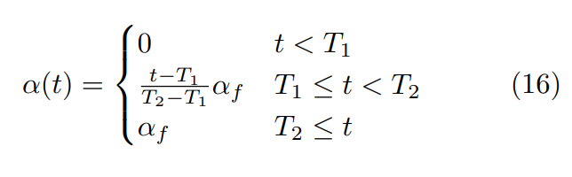
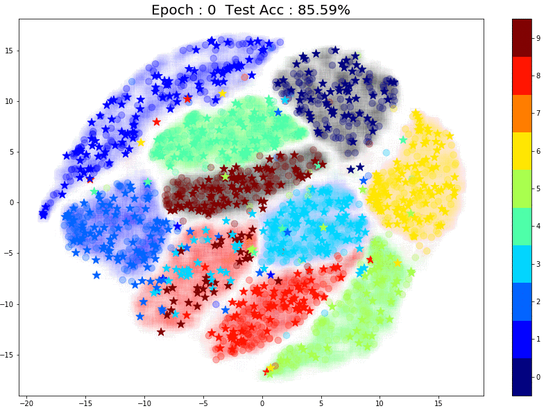
TSNE Visualization
Now let’s have a look at how the pseudo labels are being assigned at every epoch. In the plot below, there are 3 things to note:
The
faint color in the background of each cluster is the true label. This
is created using TSNE of all 60k training images (labels used)
The small circles inside each cluster are from the 1000 training images that were used in the supervised training phase.
The
small stars that keep moving are the pseudo labels that the model
assigns for the unlabeled images for each epoch. (For each epoch I used
~750 randomly sampled unlabeled images to create the plot)
TSNE Animation
Here are some things to notice:
Most
of the pseudo-labels are correct. (Stars are in clusters with the same
color) This can be attributed to the high initial test accuracy.
As
training continues, the percentage of correct pseudo labels increases.
This is reflected in the increased overall test accuracy of the model.
Here’s a plot that shows the same 750 points at Epoch 0 (left) and Epoch 140 (right). I’ve marked the points that have improved in red circles.
(Note: This TSNE plot only show 750 unlabeled samples out of 59000 pts)
Now let’s find out why pseudo labeling actually works.
4. Why does Pseudo-Labeling work?
The
goal of any Semi-Supervised Learning algorithm is to use both the
unlabeled and labeled samples to learn the underlying structure of the
data. Pseudo-Labeling is able to do this by making two important
assumptions:
Continuity Assumption (Smoothness): Points that are close to each other are more likely to share a label. (Wikipedia) In other words, small changes in input do not cause
large changes in output. This assumption allows pseudo labeling to
conclude that small changes in images like rotation, shearing, etc do
not change the label.
Cluster Assumption: The data tend to form discrete clusters, and points in the same cluster are more likely to share a label. This is a special case of the continuity assumption (Wikipedia) Another way to look at this is — the decision boundary between classes lies in the low-density region (doing so helps in generalization — similar to maximum margin classifiers like SVM).
This
is why the initial labeled data is important — it helps the model learn
the underlying cluster structure. When we assign a pseudo label in the
code, we are using the cluster structure that the model has learned to
infer labels for the unlabeled data. As the training progresses, the
learned cluster structure is improved using the unlabeled data.
If
the initial labeled data is too small in size or contains outliers,
pseudo labeling will likely assign incorrect labels to the unlabeled
points. The opposite also holds, i.e. pseudo labeling can benefit from a
classifier that is already performing well with just the labeled data.
This should make more sense in the next section when we look at scenarios where pseudo-labeling fails.
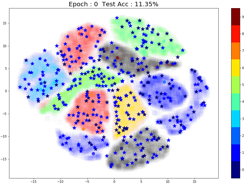
5. When does Pseudo-Labeling not work well?
Initial Labeled data is not enough to determine clusters
To
understand this scenario better, let’s run a small experiment: Instead
of using 1000 initial points let’s take the extreme case and use just 10
labeled points and see how pseudo-labeling performs:
10 Initial Labeled Points
As
expected, pseudo-labeling has almost no difference. The model itself is
as good as a random model with 10% accuracy. Since each class
effectively has just 1 point, the model is incapable of learning the
underlying structure for any class.
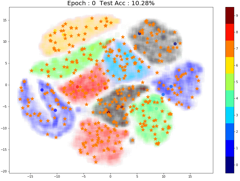
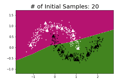
Let’s increase the number of labeled points to 20 (2 points per class) :
20 Initial Labeled Points
Now
the model is performing slightly better as it learns the structure for
some classes. Here’s something interesting — notice that pseudo-labeling
assigns the correct labels for these points (marked in red in the image
below) most likely because there are two labeled points closeby.
Small Cluster near labeled points
And finally, let’s try 50 points:
50 Labeled Points
The
performance is much better! And once again, notice the small group of
brown labeled points right in the center of the images. The points in
the same brown cluster but further away from the labeled points are
always incorrectly predicted as Aqua green (‘4’) or Orange (‘7’).
Pseudo Labels near labeled points
A few things to note:
For
all the above experiments (10,20 and 50 points) the way the labeled
points were chosen made a huge difference. Any outliers completely
changed the model’s performance and predictions for pseudo-labels. This
is a common problem with small datasets. (You can read my previous blog where I’ve discussed this in detail)
While TSNE is a great tool for visualization, we need to keep in mind that it is probabilistic and merely gives us an idea of how clusters might be distributed in higher-dimensional space.
To
conclude, both the quantity and quality of initial labeled points make a
difference when it comes to pseudo-labeling. Further, the model might
require different amounts of data for different classes to understand
that particular class’s structure.
Initial Labeled data does not include some classes
Let’s
see what happens if the labeled dataset does not contain one class (eg:
‘7’ not included in the labeled set, but the unlabeled data still
retains all classes)
After training 100 epochs on the labeled data:
Test Acc : 85.63000 | Test Loss : 1.555
And after semi-supervised training :
Epoch: 99 : Alpha Weight : 2.50000 | Test Acc : 87.98000 | Test Loss : 2.987
The
overall accuracy does increase from 85.6% to 87.98% but does not show
any improvements after that. This is obviously because the model is
unable to learn the cluster structure for the class label ‘7’.
The animations below should make these clear:
Animation for pseudo-labeling with a missing class
It’s
no surprise that pseudo-labeling struggles here as our model does not
have the capability to learn about classes that it has never seen
before. However, over the past few years, a lot of interest has been
shown in Zero-Shot Learning techniques which enable models to recognize
labels even if they do not exist in the training data.
No benefit from increased data
In
some cases, the model might not have enough complexity to take
advantage of the additional data. This usually happens when using
pseudo-labeling with conventional ML algorithms like Logistic Regression
or SVMs. When it comes to Deep Learning models, as Andrew Ng mentions
in his Coursera course — Large DL models almost always benefit from
having more data.
Andrew Ng — Coursera Deep Learning Specialization
6. Pseudo-Labeling with conventional ML algorithms
In
this section, we’ll apply the pseudo-labeling concept to Logistic
Regression. We’ll use the same MNIST dataset with 1000 labeled images,
59000 unlabeled images, and 10000 test images.
Feature Engineering
We’ll
first normalize all the images, followed by PCA decomposition from 784
dimensions to 50 dimensions. Following this, we’ll use sklearn’s PolynomialFeatures() with degree = 2 to add interaction and quadratic features. This leaves us with 1326 features per data point.
Effect of Increased Dataset size
Before
we get started on pseudo-labeling let’s check how Logistic Regression
performs when the training dataset size is slowly increased. This will
help us understand if the model can benefit from pseudo-labeling.
As
the number of samples in the training dataset increases from 100 to
1000 we see that the accuracy slowly increases. Further, it looks like
the accuracy is not stagnating and is following an upward trend. From
this, we can conclude that pseudo-labeling should give us a boost in
performance here.
Baseline Performance:
Let’s
check the test accuracy when Logistic Regression uses only the 1000
labeled images. We’ll do 10 training runs to account for any variations
in test scores.
from sklearn.linear_model import SGDClassifiertest_acc = []
for _ in range(10):
    log_reg  = SGDClassifier(loss = 'log', n_jobs = -1, alpha = 1e-5)
    log_reg.fit(x_train_poly, y_train)
    y_test_pred = log_reg.predict(x_test_poly)
    test_acc.append(accuracy_score(y_test_pred, y_test))


print('Test Accuracy: {:.2f}%'.format(np.array(test_acc).mean()*100))Output:
Test Accuracy: 90.86%
Our baseline test accuracy using Logistic Regression is 90.86%
Pseudo-Labeling Implementation:
When
working with Logistic Regression and other conventional ML algorithms
we need to use pseudo-labeling in a slightly different way, although the
concept remains the same.
Here are the steps:
We first train a classifier on our labeled train set.
Next, we use this classifier to predict the labels on a randomly sampled set from the unlabeled dataset.
We combine both the original train set and the predicted set and retrain the classifier on this new dataset.
Repeat steps 2 and 3 until all of the unlabeled data has been used.
Flowchart for Pseudo-Labeling with conventional ML Algos
This technique is slightly similar to the one mentioned in this blog.
However, here we recursively generate pseudo labels until all unlabeled
data have been used. Thresholds can also be used to ensure that pseudo
labels are generated only for points that the model is very confident
about (though this is not necessary).
Here’s the implementation as a wrapper around a sklearn estimator:
Pseudo-Labeling increased the accuracy from 90.86% to 92.42%. (Non-linear models with higher complexity like XGBoost might perform better)
Here, sample_rate is similar to alpha(t)
from the deep learning model example. Previously, alpha was used to
control the amount of unlabeled loss that was used, while in this case sample_rate controls how many unlabeled points are used in each iteration.
The sample_rate value itself is a hyperparameter that needs to be tuned based on the dataset and model (similar to T1, T2, and alpha_f). A value of 0.04 worked best for the MNIST + Logistic Regression example.
An interesting modification would be to schedule sample_rate to ramp up as the training progresses exactly similar to alpha(t).
Before we conclude, let’s look at some of the challenges in Semi-Supervised Learning in general.
7. Challenges with Semi-Supervised Learning
Combining Unlabeled Data with Labeled Data
The
primary objective of Semi-Supervised Learning is to use the unlabeled
data along with the labeled data to understand the underlying structure
of the dataset. The obvious question here is — How to utilize the
unlabeled data to achieve this purpose?
In the Pseudo-Labeling technique, we saw that a scheduled weight function ( alpha) was used to slowly combine the unlabeled data with the labeled data. However, the alpha(t)
function assumes that the model confidence increases over time and
therefore increases the unlabeled loss linearly. This need not be the
case as model predictions can sometimes be incorrect. In fact, if the
model makes several wrong unlabeled predictions, pseudo-labeling can act
like a bad feedback loop and deteriorate performance further. (Ref : Section 3.1 Arazo et al 2019 [2])
One solution for the problem above is to use probability thresholds — similar to what we did with Logistic Regression.
Other
Semi-Supervised Learning algorithms use different ways to combine the
data, for example, MixMatch uses a 2-step process for guessing the label
(for the unlabeled data) followed by MixUp data augmentation to combine
the unlabeled data with the labeled data. (Berthelot et al (2019)[3])
Data Efficiency
Another
challenge with Semi-Supervised Learning is to design algorithms that
can work with very small amounts of labeled data. As we’ve seen with
pseudo labeling, the model works best with 1000 initial labeled samples.
However, when the labeled dataset is reduced further (for eg: with 50
points), pseudo-labeling’s performance starts to drop.
Oliver et al. (2018)
[4] did a comparison of several Semi-Supervised Learning algorithms and
found that Pseudo-Labeling fails on the “two-moons” dataset while other
models like VAT and pi-model worked much better.
Source: Oliver et al (2018) [4]
As
shown in the image, VAT and Pi-Model learn a decision boundary that is
surprisingly good with just 6 labeled data points (shown in large white
and black circles). Pseudo-Labeling on the other hand completely fails
and learns a linear decision boundary instead.
I
repeated the experiment using the same model that Oliver et al. used
and found that pseudo-labeling required anywhere from 30–50 labeled
points (depending on the position of the labeled points) to learn the
underlying data structure.
Pseudo-Labeling on Two Moons Dataset. Triangles are labeled points.
To
make Semi-Supervised Learning more practical we need algorithms that
are highly data-efficient i.e. ones that can work on very small amounts
of labeled data.
8. Conclusion
Oliver et al.[4] mention: “Pseudo-labeling is a simple heuristic which is widely used in practice, likely because of its simplicity and generality” and as we’ve seen it provides a nice way to learn about Semi-Supervised Learning.
Over
the last 2–3 years, Semi-Supervised Learning for Image classification
has seen some incredible improvements. Unsupervised Data Augmentation (Xie et al (2019) [5]) has achieved 97.3% on CIFAR- 10 with just 4000 Labels. To put that into perspective, DenseNet (Huang et al (2016)[6]) achieved 96.54% on the complete CIFAR-10 dataset in 2016.
It’s
really interesting to see how the Machine Learning and Data Science
community is moving towards algorithms that either uses less labeled
data (like Semi-Supervised Learning, Zero/Few Shot Learning) or smaller
datasets altogether (like Transfer Learning). Personally, I believe
these developments are critical if we truly want to democratize
Artificial Intelligence for all.
If you have any questions feel free to connect with me. I hope you enjoyed!
Eric
Arazo, Diego Ortego, Paul Albert, Noel E. O’Connor, Kevin McGuinness.
“Pseudo-Labeling and Confirmation Bias in Deep Semi-Supervised Learning”
(https://arxiv.org/abs/1908.02983)
David
Berthelot, Nicholas Carlini, Ian Goodfellow, Nicolas Papernot, Avital
Oliver, Colin Raffel. “MixMatch: A Holistic Approach to Semi-Supervised
Learning” (https://arxiv.org/abs/1905.02249)
“Avital
Oliver, Augustus Odena, Colin Raffel, Ekin D. Cubuk, Ian J. Goodfellow.
“Realistic Evaluation of Deep Semi-Supervised Learning Algorithms” (https://arxiv.org/abs/1804.09170)
Qizhe Xie, Zihang Dai, Eduard Hovy, Minh-Thang Luong, Quoc V. Le. ”Unsupervised Data Augmentation for Consistency Training” (https://arxiv.org/abs/1904.12848)
Gao Huang, Zhuang Liu, Laurens van der Maaten, Kilian Q. Weinberger. “Densely Connected Convolutional Networks” (https://arxiv.org/abs/1608.06993)
Feature
selection is a fundamental step in many machine learning pipelines. You
dispose of a bunch of features and you want to select only the relevant
ones and to discard the others. The aim is simplifying the problem by
removing unuseful features which would introduce unnecessary noise (ever
heard of Occam?).
Boruta is a pretty smart algorithm dating back to2010 designed to automatically perform feature selection on a dataset. It was born as a package for R (this is the article that first described it). A version of Boruta for Python — called BorutaPy — exists and can be found here.
In
this post, we will see some straightforward Python code for
implementing Boruta from scratch — I believe that building something
from scratch is the best way to really understand it — and, at the end
of the post, we will see how to use BorutaPy to make our life easier.
1. It all starts with X and y
In order to see Boruta in action, let’s build a toy dataset with 3 features (age, height and weight), a target variable (income) and 5 observations.
import pandas as pd### make X and y
X = pd.DataFrame({'age': [25, 32, 47, 51, 62],
                  'height': [182, 176, 174, 168, 181],
                  'weight': [75, 71, 78, 72, 86]})
y = pd.Series([20, 32, 45, 55, 61], name = 'income')
X and y
So
the goal is to predict the income of a person knowing his/her age,
height and weight. This may seem nonsensical (at least in theory: in
practice, height has been proven to be related to salary), but in general it’s advisable not to be influenced by one’s bias.
In
a real-life situation, we would have to deal with more than 3 features
(from some hundreds to many thousands, typically). Thus, it would be
unfeasible to go through each of them and decide whether to keep it or
not. Moreover, there are relationships (such as non linear relationships
and interactions) that are not easily spotted by a human eye, not even
with accurate analysis.
Ideally, we would like to find an algorithm that is able to autonomously decide whether any given feature of X bears some predictive value about y.
2. Why Boruta?
A popular algorithm for feature selection is sklearn’s SelectFromModel.
Basically, you choose a model of convenience — capable of capturing
non-linear relationships and interactions, e.g. a random forest — and
you fit it on X and y. Then, you
extract the importance of each feature from this model and keep only
the features that are above a given threshold of importance.
This
sounds reasonable, but the weak spot of such an approach is
self-evident: who determines the threshold, and how? There is a good
deal of arbitrariness in it.
When
I first crashed into this problem, I started looking for a more robust
solution. Until I found Boruta. Boruta is a feature selection algorithm
which is statistically grounded and works extremely well even without
any specific input by the user. How is that even possible?
Boruta is based on two brilliant ideas.
2.1 The first idea: shadow features
In
Boruta, features do not compete among themselves. Instead — and this is
the first brilliant idea — they compete with a randomized version of
them.
In practice, starting from X, another dataframe is created by randomly shuffling each feature. These permuted features are called shadow features. At this point, the shadow dataframe is attached to the original dataframe to obtain a new dataframe (we will call it X_boruta), which has twice the number of columns of X.
import numpy as np### make X_shadow by randomly permuting each column of X
np.random.seed(42)
X_shadow = X.apply(np.random.permutation)
X_shadow.columns = ['shadow_' + feat for feat in X.columns]### make X_boruta by appending X_shadow to X
X_boruta = pd.concat([X, X_shadow], axis = 1)
This is how X_boruta would look like in our case:
X_boruta
Then, a random forest is fitted on X_boruta and y.
Now, we take the importance of each original features and compare it with a threshold. This time, the threshold is defined as the highest feature importance recorded among the shadow features. When the importance of a feature is higher than this threshold, this is called a “hit”. The idea is that a feature is useful only if it’s capable of doing better than the best randomized feature.
The code to reproduce this process is the following
from sklearn.ensemble import RandomForestRegressor### fit a random forest (suggested max_depth between 3 and 7)
forest = RandomForestRegressor(max_depth = 5, random_state = 42)
forest.fit(X_boruta, y)### store feature importances
feat_imp_X = forest.feature_importances_[:len(X.columns)]
feat_imp_shadow = forest.feature_importances_[len(X.columns):]### compute hits
hits = feat_imp_X > feat_imp_shadow.max()
For our toy dataset, the outcome is:
Outcome of one run
The threshold is 14% (maximum of 11%, 14% and 8%), thus 2 features made a hit, namely age and height (respectively 39% and 19%), whereas weight (8%) scored below the threshold.
Apparently, we should drop weight and get on with age and height. But should we trust this run? What if it was just an unlucky run for weight? What if instead it was just a lucky run for age and height?
This is where the second brilliant idea of Boruta comes into play.
2.2 The second idea: binomial distribution
As often happens in machine learning (in life?), the key is iteration. Not surprisingly, 20 trials are more reliable than 1 trial and 100 trials are more reliable than 20 trials.
For instance, let’s repeat for 20 times the process seen above.
### initialize hits counter
hits = np.zeros((len(X.columns)))### repeat 20 times
for iter_ in range(20):   ### make X_shadow by randomly permuting each column of X
   np.random.seed(iter_)
   X_shadow = X.apply(np.random.permutation)
   X_boruta = pd.concat([X, X_shadow], axis = 1)   ### fit a random forest (suggested max_depth between 3 and 7)
   forest = RandomForestRegressor(max_depth = 5, random_state = 42)
   forest.fit(X_boruta, y)   ### store feature importance
   feat_imp_X = forest.feature_importances_[:len(X.columns)]
   feat_imp_shadow = forest.feature_importances_[len(X.columns):]   ### compute hits for this trial and add to counter
   hits += (feat_imp_X > feat_imp_shadow.max())
This is the outcome:
Outcome of 20 runs
Now, how do we set a decision criterion? This is the second brilliant idea contained in Boruta.
Let’s take a feature (no matter if age, height or weight) and say we have absolutely no clue if it’s useful or not. What is the probability that we shall keep it? The maximum level of uncertainty about the feature is expressed by a probability of 50%, like tossing a coin. Since each independent experiment can give a binary outcome (hit or no hit), a series of n trials follows a binomial distribution.
In Python, the probability mass function of a binomial distibution can be computed as follows:
import scipy as sptrials = 20
pmf = [sp.stats.binom.pmf(x, trials, .5) for x in range(trials + 1)]
These values look like a bell:
Binomial distribution and positioning of the features
In Boruta, there is not a hard threshold between a refusal and an acceptance area. Instead, there are 3 areas:
an area of refusal (the red area): the features that end up here are considered as noise, so they are dropped;
an area of irresolution (the blue area): Boruta is indecisive about the features that are in this area;
an area of acceptance (the green area): the features that are here are considered as predictive, so they are kept.
The areas are defined by selecting the two most extreme portions of the distribution called tails of the distribution (in our example each tail accounts for 0.5% of the distribution).
So, we did 20 iterations on our toy data and ended up with some statistically grounded conclusions:
in order to predict the income of a person, age is predictive and should be kept, weight is just noise and should be dropped,
Boruta was indecisive about height: the choice is up to us, but in a conservative frame, it is advisable to keep it.
In this paragraph, we have implemented the necessary code, but a great (optimized) library for Boruta in Python exists.
3. Using BorutaPy in Python
Boruta can be installed via pip:
!pip install boruta
This is how it can be used:
from boruta import BorutaPy
from sklearn.ensemble import RandomForestRegressor
import numpy as np###initialize Boruta
forest = RandomForestRegressor(
   n_jobs = -1,
   max_depth = 5
)
boruta = BorutaPy(
   estimator = forest,
   n_estimators = 'auto',
   max_iter = 100 # number of trials to perform
)### fit Boruta (it accepts np.array, not pd.DataFrame)
boruta.fit(np.array(X), np.array(y))### print results
green_area = X.columns[boruta.support_].to_list()
blue_area = X.columns[boruta.support_weak_].to_list()print('features in the green area:', green_area)
print('features in the blue area:', blue_area)
As you can see, the features stored in boruta.support_ are the ones that at some point ended up in the acceptance area, thus you should include them in your model. The features stored in boruta.support_weak_
are the ones that Boruta didn’t manage to accept or refuse (blue area)
and the choice is up to the data scientist: these features may be
accepted or not depending on the use case.
4. Conclusion
Feature
selection is a decisive part of a machine learning pipeline: being too
conservative means introducing unnecessary noise, while being too
aggressive means throwing away useful information.
In
this post, we have seen how to use Boruta for performing a robust,
statistically grounded feature selection on your dataset. Indeed, making
substantial decisions about features is critical to ensure the success
of your predictive model.